This course enables the learners to understand the fundamental concepts and algorithms in machine learning.Its a part of KTU minor course in Machine Learning-Dr Binu V P, 9847390760
Linear regression is perhaps one of the most well known and well understood algorithms in statistics and machine learning.
Linear regression was developed in the field of statistics and is studied as a model for understanding the relationship between input and output numerical variables, but has been borrowed by machine learning. It is both a statistical algorithm and a machine learning algorithm.
Linear regression is a linear model, e.g. a model that assumes a linear relationship between the input variables ($x$) and the single output variable ($y$). More specifically, that $y$ can be calculated from a linear combination of the input variables ($x$).
When there is a single input variable ($x$), the method is referred to as simple linear regression. When there are multiple input variables, literature from statistics often refers to the method as multiple linear regression.
Different techniques can be used to prepare or train the linear regression equation from data, the most common of which is called Ordinary Least Squares. It is common to therefore refer to a model prepared this way as Ordinary Least Squares Linear Regression or just Least Squares Regression.
Linear Regression Model
The linear regression model is simple.The representation is a linear equation that combines a specific set of input values ($x$) the solution to which is the predicted output for that set of input values ($y$). As such, both the input values ($x$) and the output value are numeric.
For example, in a simple regression problem (a single x and a single y), the form of the model would be:
$y = \beta_0 + \beta_1*x$
In higher dimensions when we have more than one input ($x$), the line is called a plane or a hyper-plane. The representation therefore is the form of the equation and the specific values used for the coefficients.
It is common to talk about the complexity of a regression model like linear regression. This refers to the number of coefficients used in the model.
Learning a linear regression model means estimating the values of the coefficients used in the representation with the data that we have available.
Take note of Ordinary Least Squares because it is the most common method used in general. Also take note of Gradient Descent as it is the most common technique taught in machine learning classes.
1. Simple Linear Regression
With simple linear regression when we have a single input, we can use statistics to estimate the coefficients.
This requires that you calculate statistical properties from the data such as means, standard deviations, correlations and covariance. All of the data must be available to traverse and calculate statistics.
The key point in Simple Linear Regression is that the dependent variable must be a continuous/real value. However, the independent variable can be measured on continuous or categorical values.
Simple Linear regression algorithm has mainly two objectives:
Model the relationship between the two variables. Such as the relationship between Income and expenditure, experience and Salary, etc.
Forecasting new observations. Such as Weather forecasting according to temperature, Revenue of a company according to the investments in a year, etc.
Simple Linear Regression involves the model
$Y=\beta_0+\beta_1 X$
The ordinary least square estimate of $\beta_0$ and $\beta_1$ try to minimize the sum of squared error
$SSE(\beta_0,\beta_1)=\sum_{i=1}^{n}(Y_i-\hat{Y_i})^2$, where $\hat{Y}$ is the estimated value of $Y$
Finding the derivative of $SSE(\beta_0,\beta_1)$ with respect to $\beta_0$ and $\beta_1$ and equating them to zero and solving for $\beta_0$ and $\beta_1$ yields the optimum value
# calculating cross-deviation and deviation about x
SS_xy=np.sum((x-m_x)*(y-m_y))
SS_xx=np.sum((x-m_x)*(x-m_x))
# calculating regression coefficients
b_1 = SS_xy / SS_xx
b_0 = m_y - b_1*m_x
return (b_0, b_1)
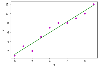
def plot_regression_line(x, y, b):
# plotting the actual points as scatter plot
plt.scatter(x, y, color = "m",marker = "o", s = 30)
# predicted response vector
y_pred = b[0] + b[1]*x
# plotting the regression line
plt.plot(x, y_pred, color = "g")
# putting labels
plt.xlabel('x')
plt.ylabel('y')
# function to show plot
plt.show()
# observations / data
x = np.array([0, 1, 2, 3, 4, 5, 6, 7, 8, 9])
y = np.array([1, 3, 2, 5, 7, 8, 8, 9, 10, 12])
# estimating coefficients
b = estimate_coef(x, y)
print("Estimated coefficients:\nb_0 = {} \
\nb_1 = {}".format(b[0], b[1]))
# plotting regression line
plot_regression_line(x, y, b)
Estimated coefficients:
b_0 = 1.2363636363636363
b_1 = 1.1696969696969697
Use the following data to construct a linear regression model for the auto insurance premium as a function of driving experience. ( university question)
2. Multiple Linear Regression(Multivariate Linear Regression)
In Simple Linear Regression, where a single Independent/Predictor(X) variable is used to model the response variable (Y). But there may be various cases in which the response variable is affected by more than one predictor variable; for such cases, the Multiple Linear Regression algorithm is used.
When we have more than one input we can use Ordinary Least Squares to estimate the values of the coefficients.
The Ordinary Least Squares procedure seeks to minimize the sum of the squared residuals. This means that given a regression line through the data we calculate the distance from each data point to the regression line, square it, and sum all of the squared errors together. This is the quantity that ordinary least squares seeks to minimize.
This approach treats the data as a matrix and uses linear algebra operations to estimate the optimal values for the coefficients. It means that all of the data must be available and you must have enough memory to fit the data and perform matrix operations.
Consider a dataset with $p$ features(or independent variables) and one response(or dependent variable).
Also, the dataset contains $n$ rows/observations. We define: $X$ (feature matrix) = a matrix of size $n \times p$ where $x_{ij}$ denotes the values of $j$th feature for $i$th observation.
#create a linear regression model and fitting the model
reg=linear_model.LinearRegression()
reg.fit(df[['area','bedrooms','age']],df.price)
print("Coefficents",reg.coef_)
print("Intercept",reg.intercept_)
print("prediction using values 5000,4,10",reg.predict([[5000,4,10]]))
outputs area bedrooms age price
0 2600 3.0 20 550000
1 3000 4.0 15 565000
2 3200 3.0 18 610000
3 3600 3.0 30 680000
4 4000 5.0 8 725000
Coefficents [ 143.625 -6762.5 337.5 ]
Intercept 173112.5
prediction using values 5000,4,10 [867562.5]
3. Gradient Descent
Gradient descent (GD) is an iterative first-order optimization algorithm used to find a local minimum/maximum of a given function. This method is commonly used in machine learning (ML) and deep learning(DL) to minimize a cost/loss function (e.g. in a linear regression).
Gradient is a slope of a curve at a given point in a specified direction.In the case of a univariate function, it is simply the first derivative at a selected point. In the case of a multivariate function, it is a vector of derivatives in each main direction (along variable axes). Because we are interested only in a slope along one axis and we don’t care about others these derivatives are called partial derivatives.
Gradient descent algorithm does not work for all functions. There are two specific requirements. A function has to be:
differentiable convex
First, what does it mean it has to be differentiable? If a function is differentiable it has a derivative for each point in its domain — not all functions meet these criteria.
differentiable functions
non differentiable functions
Next requirement — function has to be convex. For a univariate function, this means that the line segment connecting two function’s points lays on or above its curve (it does not cross it). If it does it means that it has a local minimum which is not a global one.
Another way to check mathematically if a univariate function is convex is to calculate the second derivative and check if its value is always bigger than 0.
When there are one or more inputs you can use a process of optimizing the values of the coefficients by iteratively minimizing the error of the model on your training data.
This operation is called Gradient Descent and works by starting with random values for each coefficient. The sum of the squared errors are calculated for each pair of input and output values. A learning rate is used as a scale factor and the coefficients are updated in the direction towards minimizing the error. The process is repeated until a minimum sum squared error is achieved or no further improvement is possible.
When using this method, you must select a learning rate (alpha) parameter that determines the size of the improvement step to take on each iteration of the procedure.
Gradient descent is often taught using a linear regression model because it is relatively straightforward to understand. In practice, it is useful when you have a very large data set either in the number of rows or the number of columns that may not fit into memory.
Gradient descent is an optimization algorithm used to find the values of parameters (coefficients) of a function (f) that minimizes a cost function (cost).
Gradient descent is best used when the parameters cannot be calculated analytically (e.g. using linear algebra) and must be searched for by an optimization algorithm.
For the linear regression problem the coefficients can be optimized by evaluating the cost function which is the sum of squared error
Gradient Descent Procedure
The procedure starts off with initial values for the coefficient or coefficients for the function. These could be 0.0 or a small random value.
$coefficient$ = start with a small random value
The cost of the coefficients is evaluated by plugging them into the function and calculating the cost.
$cost = evaluate(f(coefficient))$
The derivative of the cost is calculated. The derivative is a concept from calculus and refers to the slope of the function at a given point. We need to know the slope so that we know the direction (sign) to move the coefficient values in order to get a lower cost on the next iteration.
$delta = derivative(cost)$
Now that we know from the derivative which direction is downhill, we can now update the coefficient values. A learning rate parameter (alpha) must be specified that controls how much the coefficients can change on each update.
$coefficient = coefficient – (alpha * delta)$
This process is repeated until the cost of the coefficients (cost) is 0.0 or close enough to zero to be good enough.
You can see how simple gradient descent is. It does require you to know the gradient of your cost function or the function you are optimizing, but besides that, it’s very straightforward.
Gradient Descent Algorithm iteratively calculates the next point using gradient at the current position, then scales it (by a learning rate) and subtracts obtained value from the current position (makes a step). It subtracts the value because we want to minimize the function (to maximize it would be adding). This process can be written as:
$p_{n+1}=p_n-\alpha \Delta f(p_n)$
There’s an important parameter $\alpha$ which scales the gradient and thus controls the step size. In machine learning, it is called learning rate and have a strong influence on performance.The smaller learning rate the longer GD converges, or may reach maximum iteration before reaching the optimum point.If learning rate is too big the algorithm may not converge to the optimal point (jump around) or even to diverge completely.
In summary, Gradient Descent method’s steps are: choose a starting point (initialization) calculate gradient at this point make a scaled step in the opposite direction to the gradient (objective: minimise) repeat points 2 and 3 until one of the criteria is met:
The cost function involves evaluating the coefficients in the machine learning model by calculating a prediction for the model for each training instance in the data set and comparing the predictions to the actual output values and calculating a sum or average error (such as the Sum of Squared Residuals or SSR in the case of linear regression).
From the cost function a derivative can be calculated for each coefficient so that it can be updated using exactly the update equation described above.
The cost is calculated for a machine learning algorithm over the entire training data set for each iteration of the gradient descent algorithm. One iteration of the algorithm is called one batch and this form of gradient descent is referred to as batch gradient descent.
Batch gradient descent is the most common form of gradient descent described in machine learning.
Stochastic Gradient Descent for Machine Learning
Gradient descent can be slow to run on very large datasets.
Because one iteration of the gradient descent algorithm requires a prediction for each instance in the training dataset, it can take a long time when you have many millions of instances.
In situations when you have large amounts of data, you can use a variation of gradient descent called stochastic gradient descent.
In this variation, the gradient descent procedure described above is run but the update to the coefficients is performed for each training instance, rather than at the end of the batch of instances.
The first step of the procedure requires that the order of the training dataset is randomized. This is to mix up the order that updates are made to the coefficients. Because the coefficients are updated after every training instance, the updates will be noisy jumping all over the place, and so will the corresponding cost function. By mixing up the order for the updates to the coefficients, it harnesses this random walk and avoids it getting distracted or stuck.
The update procedure for the coefficients is the same as that above, except the cost is not summed over all training patterns, but instead calculated for one training pattern.
The learning can be much faster with stochastic gradient descent for very large training datasets and often you only need a small number of passes through the dataset to reach a good or good enough set of coefficients.
Note:
Optimization is a big part of machine learning.
Gradient descent is a simple optimization procedure that you can use with many machine learning algorithms.
Batch gradient descent refers to calculating the derivative from all training data before calculating an update.
Stochastic gradient descent refers to calculating the derivative from each training data instance and calculating the update immediately.
4. Regularization
There are extensions of the training of the linear model called regularization methods. These seek to both minimize the sum of the squared error of the model on the training data (using ordinary least squares) but also to reduce the complexity of the model (like the number or absolute size of the sum of all coefficients in the model).
Two popular examples of regularization procedures for linear regression are:
Lasso Regression: where Ordinary Least Squares is modified to also minimize the absolute sum of the coefficients (called L1 regularization).
Ridge Regression: where Ordinary Least Squares is modified to also minimize the squared absolute sum of the coefficients (called L2 regularization).
These methods are effective to use when there is collinearity in your input values and ordinary least squares would overfit the training data.
Lasso Regression
Linear regression refers to a model that assumes a linear relationship between input variables and the target variable.
With a single input variable, this relationship is a line, and with higher dimensions, this relationship can be thought of as a hyperplane that connects the input variables to the target variable. The coefficients of the model are found via an optimization process that seeks to minimize the sum squared error between the predictions ($\hat{y}$) and the expected target values ($y$).
$loss = \sum_{i=0}^n (y_i – \hat{y})^2$
A problem with linear regression is that estimated coefficients of the model can become large, making the model sensitive to inputs and possibly unstable. This is particularly true for problems with few observations (samples) or less samples ($n$) than input predictors ($p$) or variables (so-called $p >> n$ problems).
One approach to address the stability of regression models is to change the loss function to include additional costs for a model that has large coefficients. Linear regression models that use these modified loss functions during training are referred to collectively as penalized linear regression.
A popular penalty is to penalize a model based on the sum of the absolute coefficient values. This is called the L1 penalty. An L1 penalty minimizes the size of all coefficients and allows some coefficients to be minimized to the value zero, which removes the predictor from the model.
$L1_{penalty} = \sum_{ j=0}^p abs(\beta_j)$
An L1 penalty minimizes the size of all coefficients and allows any coefficient to go to the value of zero, effectively removing input features from the model.
This acts as a type of automatic feature selection.
A hyperparameter is used called “lambda” that controls the weighting of the penalty to the loss function. A default value of 1.0 will give full weightings to the penalty; a value of 0 excludes the penalty. Very small values of $\lambda$, such as 1e-3 or smaller, are common.
$lasso_{loss} = loss + (\lambda * L1_{penalty})$
Ridge Regression
Ridge Regression is a popular type of regularized linear regression that includes an L2 penalty. This has the effect of shrinking the coefficients for those input variables that do not contribute much to the prediction task.
One popular penalty is to penalize a model based on the sum of the squared coefficient values (beta). This is called an L2 penalty.
$L2_{penalty} = \sum_{ j=0}^p \beta_j^2$
An L2 penalty minimizes the size of all coefficients, although it prevents any coefficients from being removed from the model by allowing their value to become zero.
This penalty can be added to the cost function for linear regression and is referred to as Tikhonov regularization (after the author), or Ridge Regression more generally.
The effect of this penalty is that the parameter estimates are only allowed to become large if there is a proportional reduction in SSE. In effect, this method shrinks the estimates towards 0 as the lambda penalty becomes large (these techniques are sometimes called “shrinkage methods”).
A hyperparameter is used called “lambda” that controls the weighting of the penalty to the loss function. A default value of 1.0 will fully weight the penalty; a value of 0 excludes the penalty. Very small values of $\lambda$, such as 1e-3 or smaller are common.
Given the representation is a linear equation, making predictions is as simple as solving the equation for a specific set of inputs.
Let’s make this concrete with an example. Imagine we are predicting weight (y) from height (x). Our linear regression model representation for this problem would be:
$weight =\beta_0 +\beta_1 * height$
Where $\beta_0$ is the bias coefficient and $\beta_1$ is the coefficient for the height column. We use a learning technique to find a good set of coefficient values. Once found, we can plug in different height values to predict the weight.
For example, lets use $\beta_0 = 0.1$ and $\beta_1 = 0.5$. Let’s plug them in and calculate the weight (in kilograms) for a person with the height of 182 centimeters.
$weight = 0.1 + 0.5 * 182$
$weight = 91.1$
You can see that the above equation could be plotted as a line in two-dimensions. The $\beta_0$ is our starting point regardless of what height we have
Preparing Data For Linear Regression
Linear regression is been studied at great length, and there is a lot of literature on how your data must be structured to make best use of the model.
As such, there is a lot of sophistication when talking about these requirements and expectations which can be intimidating. In practice, you can uses these rules more as rules of thumb when using Ordinary Least Squares Regression, the most common implementation of linear regression.
Try different preparations of your data using these heuristics and see what works best for your problem.
Linear Assumption. Linear regression assumes that the relationship between your input and output is linear. It does not support anything else. This may be obvious, but it is good to remember when you have a lot of attributes. You may need to transform data to make the relationship linear (e.g. log transform for an exponential relationship).
Remove Noise. Linear regression assumes that your input and output variables are not noisy. Consider using data cleaning operations that let you better expose and clarify the signal in your data. This is most important for the output variable and you want to remove outliers in the output variable (y) if possible.
Remove Collinearity. Linear regression will over-fit your data when you have highly correlated input variables. Consider calculating pairwise correlations for your input data and removing the most correlated.
Gaussian Distributions. Linear regression will make more reliable predictions if your input and output variables have a Gaussian distribution. You may get some benefit using transforms (e.g. log or BoxCox) on you variables to make their distribution more Gaussian looking.
Rescale Inputs: Linear regression will often make more reliable predictions if you re scale input variables using standardization or normalization.
The cause of poor performance in machine learning is either overfitting or underfitting the data.
Supervised machine learning is best understood as approximating a target function (f) that maps input variables $(X)$ to an output variable $(Y).$
$Y = f(X)$
This characterization describes the range of classification and prediction problems and the machine algorithms that can be used to address them.
An important consideration in learning the target function from the training data is how well the model generalizes to new data. Generalization is important because the data we collect is only a sample, it is incomplete and noisy.
Training a deep neural network that can generalize well to new data is a challenging problem.
A model with too little capacity cannot learn the problem, whereas a model with too much capacity can learn it too well and overfit the training dataset. Both cases result in a model that does not generalize well.
A modern approach to reducing generalization error is to use a larger model that may be required to use regularization during training that keeps the weights of the model small. These techniques not only reduce overfitting, but they can also lead to faster optimization of the model and better overall performance.
Generalization in Machine Learning
In machine learning we describe the learning of the target function from training data as inductive learning.
Induction refers to learning general concepts from specific examples which is exactly the problem that supervised machine learning problems aim to solve. This is different from deduction that is the other way around and seeks to learn specific concepts from general rules.
Generalization refers to how well the concepts learned by a machine learning model apply to specific examples not seen by the model when it was learning.
The central challenge in machine learning is that we must perform well on new, previously unseen inputs — not just those on which our model was trained. The ability to perform well on previously unobserved inputs is called generalization.
The goal of a good machine learning model is to generalize well from the training data to any data from the problem domain. This allows us to make predictions in the future on data the model has never seen.
There is a terminology used in machine learning when we talk about how well a machine learning model learns and generalizes to new data, namely overfitting and underfitting.
Overfitting and underfitting are the two biggest causes for poor performance of machine learning algorithms.
We require that the model learn from known examples and generalize from those known examples to new examples in the future. We use methods like a train/test split or k-fold cross-validation only to estimate the ability of the model to generalize to new data.
Learning and also generalizing to new cases is hard.
Too little learning and the model will perform poorly on the training dataset and on new data. The model will underfit the problem. Too much learning and the model will perform well on the training dataset and poorly on new data, the model will overfit the problem. In both cases, the model has not generalized.
Underfit Model. A model that fails to sufficiently learn the problem and performs poorly on a training dataset and does not perform well on a holdout sample.
Overfit Model. A model that learns the training dataset too well, performing well on the training dataset but does not perform well on a hold out sample.
Good Fit Model. A model that suitably learns the training dataset and generalizes well to the old out dataset.
A model fit can be considered in the context of the bias-variance trade-off.
An underfit model has high bias and low variance. Regardless of the specific samples in the training data, it cannot learn the problem. An overfit model has low bias and high variance. The model learns the training data too well and performance varies widely with new unseen examples or even statistical noise added to examples in the training dataset.
Statistical Fit
In statistics, a fit refers to how well you approximate a target function.
This is good terminology to use in machine learning, because supervised machine learning algorithms seek to approximate the unknown underlying mapping function for the output variables given the input variables.
Statistics often describe the goodness of fit which refers to measures used to estimate how well the approximation of the function matches the target function.
Some of these methods are useful in machine learning (e.g. calculating the residual errors), but some of these techniques assume we know the form of the target function we are approximating, which is not the case in machine learning.
If we knew the form of the target function, we would use it directly to make predictions, rather than trying to learn an approximation from samples of noisy training data.
Overfitting in Machine Learning
Overfitting refers to a model that models the training data too well.
Overfitting happens when a model learns the detail and noise in the training data to the extent that it negatively impacts the performance of the model on new data. This means that the noise or random fluctuations in the training data is picked up and learned as concepts by the model. The problem is that these concepts do not apply to new data and negatively impact the models ability to generalize.
Overfitting is more likely with nonparametric and nonlinear models that have more flexibility when learning a target function. As such, many nonparametric machine learning algorithms also include parameters or techniques to limit and constrain how much detail the model learns.
For example, decision trees are a nonparametric machine learning algorithm that is very flexible and is subject to overfitting training data. This problem can be addressed by pruning a tree after it has learned in order to remove some of the detail it has picked up.
Underfitting in Machine Learning
Underfitting refers to a model that can neither model the training data nor generalize to new data.
An underfit machine learning model is not a suitable model and will be obvious as it will have poor performance on the training data.
Underfitting is often not discussed as it is easy to detect given a good performance metric. The remedy is to move on and try alternate machine learning algorithms. Nevertheless, it does provide a good contrast to the problem of overfitting.
A Good Fit in Machine Learning
Ideally, you want to select a model at the sweet spot between underfitting and overfitting.
This is the goal, but is very difficult to do in practice.
To understand this goal, we can look at the performance of a machine learning algorithm over time as it is learning a training data. We can plot both the skill on the training data and the skill on a test dataset we have held back from the training process.
Over time, as the algorithm learns, the error for the model on the training data goes down and so does the error on the test dataset. If we train for too long, the performance on the training dataset may continue to decrease because the model is overfitting and learning the irrelevant detail and noise in the training dataset. At the same time the error for the test set starts to rise again as the model’s ability to generalize decreases.
The sweet spot is the point just before the error on the test dataset starts to increase where the model has good skill on both the training dataset and the unseen test dataset.
You can perform this experiment with your favorite machine learning algorithms. This is often not useful technique in practice, because by choosing the stopping point for training using the skill on the test dataset it means that the testset is no longer “unseen” or a standalone objective measure. Some knowledge (a lot of useful knowledge) about that data has leaked into the training procedure.
There are two additional techniques you can use to help find the sweet spot in practice: resampling methods and a validation dataset.
How To Limit Overfitting
Both overfitting and underfitting can lead to poor model performance. But by far the most common problem in applied machine learning is overfitting.
Overfitting is such a problem because the evaluation of machine learning algorithms on training data is different from the evaluation we actually care the most about, namely how well the algorithm performs on unseen data.
There are two important techniques that you can use when evaluating machine learning algorithms to limit overfitting:
Use a resampling technique to estimate model accuracy.
Hold back a validation dataset.
The most popular resampling technique is k-fold cross validation. It allows you to train and test your model k-times on different subsets of training data and build up an estimate of the performance of a machine learning model on unseen data.
A validation dataset is simply a subset of your training data that you hold back from your machine learning algorithms until the very end of your project. After you have selected and tuned your machine learning algorithms on your training dataset you can evaluate the learned models on the validation dataset to get a final objective idea of how the models might perform on unseen data.
Using cross validation is a gold standard in applied machine learning for estimating model accuracy on unseen data. If you have the data, using a validation dataset is also an excellent practice.
What is R-squared?
R squared or Coefficient of determination, or $R^2$ is a measure that provides information about the goodness of fit of the regression model. In simple terms, it is a statistical measure that tells how well the plotted regression line fits the actual data. R squared measures how much the variation is there in predicted and actual values in the regression model.
What is the significance of R squared
R-squared values range from 0 to 1, usually expressed as a percentage from 0% to 100%.
And this value of R square tells you how well the data fits the line you’ve drawn.
The higher the model’s R-Squared value, the better the regression line fits the data.
Note: R-squared values very close to 1 are likely overfitting of the model and should be avoided.
So if the model value is close to 0, then the model is not a good fit
A good model should have an R-squared greater than 0.8.
When to Use R Squared
Linear regression is a powerful tool for predicting future events, and the r-squared statistic measures how accurate your predictions are. But when should you use r-squared?
Both independent and dependent variables must be continuous.
When the independent and dependent variables have linear relationship (+ve or -ve) between them.
How to calculate R squared in linear regression?
The deviation of an actual value from the mean is therefore calculated as the sum of the squared distances of the individual points from the mean. This is also called the total sum of squares (SST). SST is also called total error. Mathematically, SST is expressed as:
$SST=\sum_{i=1}^n (y_i-\bar{y})$
where $\bar{y}$ represents the average(mean) and $y_i$ represents the actual value.
The total variation of the actual values from the regression line is expressed as the sum of the squared distances between the predicted values from the regression line, also known as the Residual sum of squared error (SSR). SSR is sometimes called explanatory error or explanatory variance. Mathematically, SSR is expressed as
$SSR=\sum_{i=1}^n (y_i-\hat{y_i})$
$\hat{y_i}$ represents the predicted value and $y_i$ represents the actual value.
The formula to calculate $R- Squared$ is
$R-squared=1-\frac{SSR}{SST}$
where: $SSR$ is the sum of squared residuals (i.e., the sum of squared errors) $SST$ is the total sum of squares (i.e., the sum of squared deviations from the mean)
Limitations of Using R Squared
R squared can be misleading if you’re not careful. For example, if you have a lot of noise in your data, your r-squared value will inflate. In other words, it’ll look like your model needs to do a better job of predicting the data when in reality, it’s not.
R-squared values don’t help in case we have categorical variables.
Logistic Regression is one of the basic and popular algorithms to solve a classification problem. It is named ‘Logistic Regression’ because its underlying technique is quite the same as Linear Regression. The term “Logistic” is taken from the Logit function that is used in this method of classification.
The logistic function, also called the sigmoid function was developed by statisticians to describe properties of population growth in ecology, rising quickly and maxing out at the carrying capacity of the environment. It’s an S-shaped curve that can take any real-valued number and map it into a value between 0 and 1, but never exactly at those limits.
$1 / (1 + e^{-value})$
We identify the problem as a classification problem when independent variables are continuous in nature and the dependent variable is in categorical form i.e. in classes like positive class and negative class. The real-life example of classification example would be, to categorize the mail as spam or not spam, to categorize the tumor as malignant or benign, and to categorize the transaction as fraudulent or genuine. All these problem’s answers are in categorical form i.e. Yes or No. and that is why they are two-class classification problems.
Although, sometimes we come across more than 2 classes, and still it is a classification problem. These types of problems are known as multi-class classification problems.
Suppose we have data of tumor size vs its malignancy. As it is a classification problem, if we plot, we can see, all the values will lie on 0 and 1. And if we fit the best-found regression line, by assuming the threshold at 0.5, we can do line pretty reasonable job.We can decide the point on the x-axis from where all the values lie to its left side are considered as a negative class and all the values lie to its right side are positive class.
But what if there is an outlier in the data. Things would get pretty messy. For example, for 0.5 thresholds,
If we fit the best-found regression line, it still won’t be enough to decide any point by which we can differentiate classes. It will put some positive class examples into negative class. The green dotted line (Decision Boundary) is dividing malignant tumors from benign tumors but the line should have been at a yellow line which is clearly dividing the positive and negative examples. So just a single outlier is disturbing the whole linear regression predictions. And that is where logistic regression comes into the picture.
From this example, it can be inferred that linear regression is not suitable for classification problem. Linear regression is unbounded, and this brings logistic regression into picture. Their value strictly ranges from 0 to 1.
Data is fit into linear regression model, which then be acted upon by a logistic function predicting the target categorical dependent variable.This justifies the name ‘logistic regression’.
As discussed earlier, to deal with outliers, Logistic Regression uses the Sigmoid function.
An explanation of logistic regression can begin with an explanation of the standard logistic function. The logistic function is a Sigmoid function, which takes any real value between zero and one. It is defined as
$\sigma (t)=\frac{e^t}{e^t+1}=\frac{1}{1+e^{-t}}$
Let’s consider $t$ as a linear function in a univariate regression model.
$t=\beta_0+\beta_1 x$
So the Logistic Equation will become
$\sigma (x)=\frac{1}{1+e^{-(\beta_0+\beta_1x)}}$
Now, when the logistic regression model comes across an outlier, it will take care of it.
Types of Logistic Regression
1. Binary Logistic Regression
The categorical response has only two 2 possible outcomes. Example: Spam or Not
2. Multinomial Logistic Regression
Three or more categories without ordering. Example: Predicting which food is preferred more (Veg, Non-Veg, Vegan)
3. Ordinal Logistic Regression
Three or more categories with ordering. Example: Movie rating from 1 to 5
Decision Boundary
To predict which class a data belongs, a threshold can be set. Based upon this threshold, the obtained estimated probability is classified into classes.
Say, if $predicted-value ≥ 0.5$, then classify email as spam else as not spam.
Decision boundary can be linear or non-linear. Polynomial order can be increased to get complex decision boundary.
For the binary classification problem , the decision boundary is always linear.
The fundamental application of logistic regression is to determine a decision boundary for a binary classification problem. Although the baseline is to identify a binary decision boundary, the approach can be very well applied for scenarios with multiple classification classes or multi-class classification.
Cost Function ( Cross Entropy Loss Function)
Linear regression uses Least Squared Error as loss function that gives a convex graph and then we can complete the optimization by finding its vertex as global minimum. However, it’s not an option for logistic regression anymore. Since the hypothesis is changed, Least Squared Error will result in a non-convex graph with local minimums by calculating with sigmoid function applied on raw model output.
if $h(\beta)=sigmoid(\beta_0+\beta_1x)$
$cost(h_\beta(x),y_{actual})=-log(h_{\beta}(x))$ if $y=1$
$cost(h_\beta(x),y_{actual})= -log(1-h_{\beta}(x))$ if $y=0$
Intuitively, we want to assign more punishment when predicting 1 while the actual is 0 and when predict 0 while the actual is 1. The loss function of logistic regression is doing this exactly which is called Logistic Loss. See as below. If y = 1, looking at the plot below on left(blue), when prediction = 1, the cost = 0, when prediction = 0, the learning algorithm is punished by a very large cost. Similarly, if y = 0, the plot on right shows(red), predicting 0 has no punishment but predicting 1 has a large value of cost.
Another advantage of this loss function is that although we are looking at it by $y = 1$ and $y = 0$ separately, it can be written as one single formula which brings convenience for calculation:
So the cost function of the model is the summation from all training data samples:
Logistic regression is a classification algorithm.
It is intended for datasets that have numerical input variables and a categorical target variable that has two values or classes. Problems of this type are referred to as binary classification problems.
Logistic regression is designed for two-class problems, modeling the target using a binomial probability distribution function. The class labels are mapped to 1 for the positive class or outcome and 0 for the negative class or outcome. The fit model predicts the probability that an example belongs to class 1.
By default, logistic regression cannot be used for classification tasks that have more than two class labels, so-called multi-class classification.
Instead, it requires modification to support multi-class classification problems.
One popular approach for adapting logistic regression to multi-class classification problems is to split the multi-class classification problem into multiple binary classification problems and fit a standard logistic regression model on each subproblem. Techniques of this type include one-vs-rest and one-vs-one wrapper models.
An alternate approach involves changing the logistic regression model to support the prediction of multiple class labels directly. Specifically, to predict the probability that an input example belongs to each known class label.
The probability distribution that defines multi-class probabilities is called a multinomial probability distribution. A logistic regression model that is adapted to learn and predict a multinomial probability distribution is referred to as Multinomial Logistic Regression. Similarly, we might refer to default or standard logistic regression as Binomial Logistic Regression.
Binomial Logistic Regression: Standard logistic regression that predicts a binomial probability (i.e. for two classes) for each input example.
Multinomial Logistic Regression: Modified version of logistic regression that predicts a multinomial probability (i.e. more than two classes) for each input example.
Using iris data set
from sklearn import datasets from sklearn.linear_model import LogisticRegression
iris = datasets.load_iris()
X = iris['data'] y = iris['target']
logit = LogisticRegression(max_iter = 10000)
print(logit.fit(X,y))
print(logit.score(X,y))
Advantages of Logistic Regression
The advantages of the logistic regression are as follows:
1. Logistic Regression is very easy to understand. 2. It requires less training. 3. It performs well for simple datasets as well as when the data set is linearly separable. 4. It doesn’t make any assumptions about the distributions of classes in feature space.
5. A Logistic Regression model is less likely to be over-fitted but it can overfit in high dimensional datasets. To avoid over-fitting these scenarios, One may consider regularization.
Disadvantages of Logistic Regression
The disadvantages of the logistic regression are as follows:
1. Sometimes a lot of Feature Engineering is required.
2. If the independent features are correlated with each other it may affect the performance of the classifier.
3. It is quite sensitive to noise and overfitting.
4. Logistic Regression should not be used if the number of observations is lesser than the number of features, otherwise, it may lead to overfitting.
5. By using Logistic Regression, non-linear problems can’t be solved because it has a linear decision surface. But in real-world scenarios, the linearly separable data is rarely found.
Classification Performance
Binary classification has four possible types of results:
You usually evaluate the performance of your classifier by comparing the actual and predicted outputs and counting the correct and incorrect predictions.
The most straightforward indicator of classification accuracy is the ratio of the number of correct predictions to the total number of predictions (or observations)(score). Other indicators of binary classifiers include the following:
The positive predictive value is the ratio of the number of true positives to the sum of the numbers of true and false positives.(Precision)
The negative predictive value is the ratio of the number of true negatives to the sum of the numbers of true and false negatives.
The sensitivity (also known as Recall or true positive rate) is the ratio of the number of true positives to the number of actual positives.
The specificity (or true negative rate) is the ratio of the number of true negatives to the number of actual negatives.
Accuracy is just the ratio of correct results to all the results of a test.
F1-scoreis one of the most important evaluation metrics in machine learning. It elegantly sums up the predictive performance of a model by combining two otherwise competing metrics — precision and recall.
Confusion Matrix:A confusion matrix is a matrix that is used to define the performance of a classification algorithm. A confusion matrix visualizes and summarizes the performance of a classification algorithm.
Example:
Definitions:
Patient: positive for disease ( sick)
Healthy: negative for disease
True positive (TP)= the number of cases correctly identified as patient
False positive (FP) = the number of cases incorrectly identified as patient
True negative (TN) = the number of cases correctly identified as healthy
False negative (FN) = the number of cases incorrectly identified as healthy
Confusion Matrix
Positive predictive value: ( Precision)
Positive predictive value is the proportion of cases giving positive test results who are already patients . It is the ratio of patients truly diagnosed as positive to all those who had positive test results (including healthy subjects who were incorrectly diagnosed as patient). This characteristic can predict how likely it is for someone to truly be patient, in case of a positive test result.
Positive predictive value=$\frac{TP}{TP+FP}$
Precision attempts to answer the following question: What proportion of positive identifications was actually correct?
Negative predictive value:
Negative predictive value is the proportion of the cases giving negative test results who are already healthy. It is the ratio of subjects truly diagnosed as negative to all those who had negative test results (including patients who were incorrectly diagnosed as healthy). This characteristic can predict how likely it is for someone to truly be healthy, in case of a negative test result.
Negative predictive value=$\frac{TN}{TN+FN}$
Sensitivity :( Recall)
The proportion of people with the disease who tested positive compared to the number of all the people with the disease, regardless of their test result.
To calculate sensitivity, we'll need:Number of true positive cases (TP); and Number of false negative cases (FN).
$Sensitivity = \frac{TP} {(TP + FN)}$
Recall attempts to answer the following question: What proportion of actual positives was identified correctly?
Specificity:
The proportion of healthy people that tested negative compared to the total number of people without the disease, no matter their test result.
To calculate specificity, we'll need:Number of true negative cases (TN); and Number of false positive cases (FP).
$Specificity = \frac{TN }{ (FP + TN)}$
Accuracy
From all the classes (positive and negative), how many of them we have predicted correctly.
Precision measures the extent of error caused by False Positives (FPs) whereas recall measures the extent of error caused by False Negatives (FNs). Therefore, to decide which metric to use, we should assess the relative impact of these two types of errors on our use-case. Thus, the key question we should be asking is:
“Which type of error — FPs or FNs — is more undesirable for our use-case?”
It is also possible that for your use-case, you assess that the errors caused by FPs and FNs are (almost) equally undesirable. Hence, you may wish for a model to have as few FPs and FNs as possible. Put differently, you would want to maximize both precision and recall. In practice, it is not possible to maximize both precision and recall at the same time because of the trade-off between precision and recall.
Increasing precision will decrease recall, and vice versa.
So, given pairs of precision and recall values for different models, how would you compare and decide which is the best? The answer is F1-score.
By definition, F1-score is the harmonic mean of precision and recall. It combines precision and recall into a single number using the following formula:
This formula can also be equivalently written as, $F1-score=2 \times \frac{Precision \times Recall}{ Precision + Recall }$
Notice that F1-score takes both precision and recall into account, which also means it accounts for both FPs and FNs. The higher the precision and recall, the higher the F1-score. F1-score ranges between 0 and 1. The closer it is to 1, the better the model.
Suppose we have trained three different models for cancer prediction, and each model has different precision and recall values.
Figure courtesy:towards data science
If we assess that errors caused by FPs are more undesirable, then we will select a model based on precision and choose Model C.
If we assess that errors caused by FNs are more undesirable, then we will select a model based on recall and choose Model B.
However, if we assess that both types of errors are undesirable, then we will select a model based on F1-score and choose Model A.
So, the takeaway here is that the model you select depends greatly on the evaluation metric you choose, which in turn depends on the relative impacts of errors of FPs and FNs in your use-case.
The most suitable indicator depends on the problem of interest.
Support
Support is the number of actual occurrences of the class in the specified dataset. Imbalanced support in the training data may indicate structural weaknesses in the reported scores of the classifier and could indicate the need for stratified sampling or rebalancing. Support doesn’t change between models but instead diagnoses the evaluation process.
Example: ( university question)
Suppose 10000 patients get tested for flu; out of them, 9000 are actually healthy and 1000 are actually sick. For the sick people, a test was positive for 620 and negative for 380. For healthy people, the same test was positive for 180 and negative for 8820. Construct a confusion matrix for the data and compute the accuracy, precision and recall for the data
Example:
Consider a two-class classification problem of predicting whether a photograph contains a man or a woman. Suppose we have a test dataset of 10 records with expected outcomes and a set of predictions from our classification algorithm. Compute the confusion matrix, accuracy, precision, recall, sensitivity and specificity on the following data.
$\begin{vmatrix} No & Actual & Predicted \\ 1 & man & woman \\ 2& man & man\\ 3&woman & woman \\ 4& man & man\\ 5&man&woman\\ 6&woman & woman \\ 7&woman&man \\ 8&man&man\\ 9&man&woman\\ 10&woman & woman\\ \end{vmatrix}$
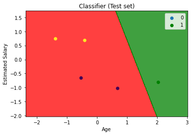
User Database – This dataset contains information about users from a company’s database. It contains information about UserID, Gender, Age, EstimatedSalary, and Purchased. We are using this dataset for predicting whether a user will purchase the company’s newly launched product or not.
Let us make the Logistic Regression model, predicting whether a user will purchase the product or not.
import pandas as pd
import numpy as np
import matplotlib.pyplot as plt
dataset = pd.read_csv("User_Data.csv")
# input
x = dataset.iloc[:, [2, 3]].values
# output
y = dataset.iloc[:, 4].values
from sklearn.model_selection import train_test_split
xtrain, xtest, ytrain, ytest = train_test_split(x, y, test_size=0.25, random_state=0)
from sklearn.preprocessing import StandardScaler
sc_x = StandardScaler()
xtrain = sc_x.fit_transform(xtrain)
xtest = sc_x.transform(xtest)
from sklearn.linear_model import LogisticRegression
To solve a problem on a computer, we need an algorithm. An algorithm is a sequence of instructions that should be carried out to transform the input to output. For example, one can devise an algorithm for sorting. The input is a set of numbers and the output is their ordered list. For the same task, there may be various algorithms and we may be interested in finding the most efficient one, requiring the least number of instructions or memory or both. For some tasks, however, we do not have an algorithm—for example,to tell spam emails from legitimate emails. We know what the input is:an email document that in the simplest case is a file of characters. We know what the output should be: a yes/no output indicating whether the message is spam or not. We do not know how to transform the input to the output. What can be considered spam changes in time and from individual to individual.We can easily compile thousands of example messages some of which we know to be spam and what we want is t...
Module-1 (Overview of machine learning) Machine learning paradigms-supervised, semi-supervised, unsupervised, reinforcement learning. Basics of parameter estimation - maximum likelihood estimation(MLE) and maximum a posteriori estimation(MAP). Introduction to Bayesian formulation. Module-2 (Supervised Learning) Regression - Linear regression with one variable, Linear regression with multiple variables, solution using gradient descent algorithm and matrix method, basic idea of overfitting in regression. Linear Methods for Classification- Logistic regression, Perceptron, Naive Bayes, Decision tree algorithm ID3. Module-3 (Neural Networks (NN) and Support Vector Machines (SVM)) NN - Multilayer feed forward network, Activation functions (Sigmoid, ReLU, Tanh), Backpropagation algorithm. SVM - Introduction, Maximum Margin Classification, Mathematics behind Maximum Margin Classification, Maximum Margin linear separators, soft margin SVM classifier, non-linear SVM, Kernels ...


 Note: The below code use scipy stats module linregress method
 Image credit: towards data science
 But what if there is an outlier in the data. Things would get pretty messy. For example, for 0.5 thresholds,


 Example:


Comments
Post a Comment