Decision Trees-ID3 Algorithm

 Decision Trees

Decision trees are very popular for predictive modeling and perform both, classification and regression. Decision trees are highly interpretable and provide a foundation for more complex algorithms, e.g., random forest.

Example: Suppose there is a candidate who has a job offer and wants to decide whether he should accept the offer or Not. So, to solve this problem, the decision tree starts with the root node (Salary attribute by ASM). The root node splits further into the next decision node (distance from the office) and one leaf node based on the corresponding labels. The next decision node further gets split into one decision node (Cab facility) and one leaf node. Finally, the decision node splits into two leaf nodes (Accepted offers and Declined offer). Consider the below diagram:

It is a tree-structured classifier, where internal nodes represent the features of a dataset, branches represent the decision rules and each leaf node represents the outcome.

In a Decision tree, there are two nodes, which are the Decision Node and Leaf Node. Decision nodes are used to make any decision and have multiple branches, whereas Leaf nodes are the output of those decisions and do not contain any further branches.

The decisions or the test are performed on the basis of features of the given dataset.

It is a graphical representation for getting all the possible solutions to a problem/decision based on given conditions.

It is called a decision tree because, similar to a tree, it starts with the root node, which expands on further branches and constructs a tree-like structure.

How does the Decision Tree algorithm Work?

In a decision tree, for predicting the class of the given dataset, the algorithm starts from the root node of the tree. This algorithm compares the values of root attribute with the record (real dataset) attribute and, based on the comparison, follows the branch and jumps to the next node.

For the next node, the algorithm again compares the attribute value with the other sub-nodes and move further. It continues the process until it reaches the leaf node of the tree. The complete process can be better understood using the below algorithm:

Step-1: Begin the tree with the root node, says S, which contains the complete dataset.
Step-2: Find the best attribute in the dataset using Attribute Selection Measure (ASM).
Step-3: Divide the S into subsets that contains possible values for the best attributes.
Step-4: Generate the decision tree node, which contains the best attribute.
Step-5: Recursively make new decision trees using the subsets of the dataset created in step -3

Continue this process until a stage is reached where you cannot further classify the nodes and called the final node as a leaf node.

The two decision tree algorithms  are CART (Classification and Regression Trees) and ID3 (Iterative Dichotomiser 3).

Why use Decision Trees?

There are various algorithms in Machine learning, so choosing the best algorithm for the given dataset and problem is the main point to remember while creating a machine learning model. Below are the two reasons for using the Decision tree:

Decision Trees usually mimic human thinking ability while making a decision, so it is easy to understand.

The logic behind the decision tree can be easily understood because it shows a tree-like structure.

Attribute Selection Measures

While implementing a Decision tree, the main issue arises that how to select the best attribute for the root node and for sub-nodes. So, to solve such problems there is a technique which is called as Attribute selection measure or ASM. By this measurement, we can easily select the best attribute for the nodes of the tree. There are two popular techniques for ASM, which are:

Information Gain
Gini Index

1. Information Gain:

Information gain is the measurement of changes in entropy after the segmentation of a dataset based on an attribute.

It calculates how much information a feature provides us about a class.
According to the value of information gain, we split the node and build the decision tree.
A decision tree algorithm always tries to maximize the value of information gain, and a node/attribute having the highest information gain is split first. It can be calculated using the below formula:

Information Gain= Entropy(S)- [(Weighted Avg) *Entropy(each feature)]

Entropy: Entropy is a metric to measure the impurity in a given attribute. It specifies randomness in data. Entropy can be calculated as:

$Entropy(S)= -P(yes)log_2 P(yes)- P(no) log_2 P(no)$

Where,
S= Total number of samples
P(yes)= probability of yes
P(no)= probability of no

2. Gini Index:

Gini index is a measure of impurity or purity used while creating a decision tree in the CART(Classification and Regression Tree) algorithm.

An attribute with the low Gini index should be preferred as compared to the high Gini index.

It only creates binary splits, and the CART algorithm uses the Gini index to create binary splits.

Gini index can be calculated using the below formula:

$Gini Index= 1- \sum_i P_i^2$

Lets consider an example of information gain which is used in ID3 algorithm

Entropy comes from information theory. More the entropy more the information content.

What is the entropy of a group in which all examples belong to the same class?

$entropy = -1 log_21 = 0$
not a good training set for learning

What is the entropy of a group with 50% in either class?

$entropy = -0.5 log_20.5 –0.5 log_20.5 =1$
good training set for learning

We want to determine which attribute in a given set of training feature vectors is most useful for discriminating between the classes to be learned.

Information gain tells us how important a given attribute of the feature vectors is.

We will use it to decide the ordering of attributes in the nodes of a decision tree.

ID3 Algorithm uses information gain to construct a decision tree

ID3 

ID3 stands for Iterative Dichotomiser 3 and is named such because the algorithm iteratively (repeatedly) dichotomizes(divides) features into two or more groups at each step.

Invented by Ross Quinlan, ID3 uses a top-down greedy approach to build a decision tree. In simple words, the top-down approach means that we start building the tree from the top and the greedy approach means that at each iteration we select the best feature at the present moment to create a node.

Most generally ID3 is only used for classification problems with nominal features only.

Dataset description

Consider  a sample dataset of COVID-19 infection. A preview of the entire dataset is shown below.

+----+-------+-------+------------------+----------+
| ID | Fever | Cough | Breathing issues | Infected |
+----+-------+-------+------------------+----------+
| 1  | NO    | NO    | NO               | NO       |
+----+-------+-------+------------------+----------+
| 2  | YES   | YES   | YES              | YES      |
+----+-------+-------+------------------+----------+
| 3  | YES   | YES   | NO               | NO       |
+----+-------+-------+------------------+----------+
| 4  | YES   | NO    | YES              | YES      |
+----+-------+-------+------------------+----------+
| 5  | YES   | YES   | YES              | YES      |
+----+-------+-------+------------------+----------+
| 6  | NO    | YES   | NO               | NO       |
+----+-------+-------+------------------+----------+
| 7  | YES   | NO    | YES              | YES      |
+----+-------+-------+------------------+----------+
| 8  | YES   | NO    | YES              | YES      |
+----+-------+-------+------------------+----------+
| 9  | NO    | YES   | YES              | YES      |
+----+-------+-------+------------------+----------+
| 10 | YES   | YES   | NO               | YES      |
+----+-------+-------+------------------+----------+
| 11 | NO    | YES   | NO               | NO       |
+----+-------+-------+------------------+----------+
| 12 | NO    | YES   | YES              | YES      |
+----+-------+-------+------------------+----------+
| 13 | NO    | YES   | YES              | NO       |
+----+-------+-------+------------------+----------+
| 14 | YES   | YES   | NO               | NO       |
+----+-------+-------+------------------+----------+

The columns are self-explanatory. Y and N stand for Yes and No respectively. The values or classes in Infected column Y and N represent Infected and Not Infected respectively.

The columns used to make decision nodes viz. ‘Breathing Issues’, ‘Cough’ and ‘Fever’ are called feature columns or just features and the column used for leaf nodes i.e. ‘Infected’ is called the target column.

Metrics in ID3

As mentioned previously, the ID3 algorithm selects the best feature at each step while building a Decision tree.

Before you ask, the answer to the question: ‘How does ID3 select the best feature?’ is that ID3 uses Information Gain or just Gain to find the best feature.

Information Gain calculates the reduction in the entropy and measures how well a given feature separates or classifies the target classes. The feature with the highest Information Gain is selected as the best one.

In simple words, Entropy is the measure of disorder and the Entropy of a dataset is the measure of disorder in the target feature of the dataset.

In the case of binary classification (where the target column has only two types of classes) entropy is 0 if all values in the target column are homogenous(similar) and will be 1 if the target column has equal number values for both the classes.

We denote our dataset as S, entropy is calculated as:

Entropy(S) = - ∑ pᵢ * log₂(pᵢ) ; i = 1 to n
where,
n is the total number of classes in the target column (in our case n = 2 i.e YES and NO)

pᵢ is the probability of class ‘i’ or the ratio of “number of rows with class i in the target column” to the “total number of rows” in the dataset.

Information Gain for a feature column A is calculated as:

IG(S, A) = Entropy(S) - ∑((|Sᵥ| / |S|) * Entropy(Sᵥ))

where Sᵥ is the set of rows in S for which the feature column A has value v, |Sᵥ| is the number of rows in Sᵥ and likewise |S| is the number of rows in S.

ID3 Steps

1. Calculate the Information Gain of each feature.
2. Considering that all rows don’t belong to the same class, split the dataset $S$ into subsets using the feature for which the Information Gain is maximum.
3. Make a decision tree node using the feature with the maximum Information gain.
4. If all rows belong to the same class, make the current node as a leaf node with the class as its label.
5. Repeat for the remaining features until we run out of all features, or the decision tree has all leaf nodes.
6. Learn the ID3 algorithm with an example here

Implementation on our Dataset

As stated in the previous section the first step is to find the best feature i.e. the one that has the maximum Information Gain(IG). We’ll calculate the IG for each of the features now, but for that, we first need to calculate the entropy of S

From the total of 14 rows in our dataset S, there are 8 rows with the target value YES and 6 rows with the target value NO. The entropy of S is calculated as:

Entropy(S) = — (8/14) * log₂(8/14) — (6/14) * log₂(6/14) = 0.99

Note: If all the values in our target column are same the entropy will be zero (meaning that it has no or zero randomness).

We now calculate the Information Gain for each feature:

IG calculation for Fever:

In this(Fever) feature there are 8 rows having value YES and 6 rows having value NO.As shown below, in the 8 rows with YES for Fever, there are 6 rows having target value YES and 2 rows having target value NO.

+-------+-------+------------------+----------+
| Fever | Cough | Breathing issues | Infected |
+-------+-------+------------------+----------+
| YES   | YES   | YES              | YES      |
+-------+-------+------------------+----------+
| YES   | YES   | NO               | NO       |
+-------+-------+------------------+----------+
| YES   | NO    | YES              | YES      |
+-------+-------+------------------+----------+
| YES   | YES   | YES              | YES      |
+-------+-------+------------------+----------+
| YES   | NO    | YES              | YES      |
+-------+-------+------------------+----------+
| YES   | NO    | YES              | YES      |
+-------+-------+------------------+----------+
| YES   | YES   | NO               | YES      |
+-------+-------+------------------+----------+
| YES   | YES   | NO               | NO       |
+-------+-------+------------------+----------+

As shown below, in the 6 rows with NO, there are 2 rows having target value YES and 4 rows having target value NO.

+-------+-------+------------------+----------+
| Fever | Cough | Breathing issues | Infected |
+-------+-------+------------------+----------+
| NO    | NO    | NO               | NO       |
+-------+-------+------------------+----------+
| NO    | YES   | NO               | NO       |
+-------+-------+------------------+----------+
| NO    | YES   | YES              | YES      |
+-------+-------+------------------+----------+
| NO    | YES   | NO               | NO       |
+-------+-------+------------------+----------+
| NO    | YES   | YES              | YES      |
+-------+-------+------------------+----------+
| NO    | YES   | YES              | NO       |
+-------+-------+------------------+----------+

The block, below, demonstrates the calculation of Information Gain for Fever.

# total rows
|S| = 14For v = YES, |Sᵥ| = 8
Entropy(Sᵥ) = - (6/8) * log₂(6/8) - (2/8) * log₂(2/8) = 0.81For v = NO, |Sᵥ| = 6
Entropy(Sᵥ) = - (2/6) * log₂(2/6) - (4/6) * log₂(4/6) = 0.91# Expanding the summation in the IG formula:
IG(S, Fever) = Entropy(S) - (|Sʏᴇs| / |S|) * Entropy(Sʏᴇs) - 
(|Sɴᴏ| / |S|) * Entropy(Sɴᴏ)∴ IG(S, Fever) = 0.99 - (8/14) * 0.81 - (6/14) * 0.91 = 0.13

Next, we calculate the IG for the features “Cough” and “Breathing issues”.You can use this free online tool to calculate the Information Gain.

IG(S, Cough) = 0.04
IG(S, BreathingIssues) = 0.40

Since the feature Breathing issues have the highest Information Gain it is used to create the root node.

Hence, after this initial step our tree looks like this: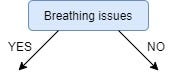

Next, from the remaining two unused features, namely, Fever and Cough, we decide which one is the best for the left branch of Breathing Issues.Since the left branch of Breathing Issues denotes YES, we will work with the subset of the original data i.e the set of rows having YES as the value in the Breathing Issues column. These 8 rows are shown below:

+-------+-------+------------------+----------+
| Fever | Cough | Breathing issues | Infected |
+-------+-------+------------------+----------+
| YES   | YES   | YES              | YES      |
+-------+-------+------------------+----------+
| YES   | NO    | YES              | YES      |
+-------+-------+------------------+----------+
| YES   | YES   | YES              | YES      |
+-------+-------+------------------+----------+
| YES   | NO    | YES              | YES      |
+-------+-------+------------------+----------+
| YES   | NO    | YES              | YES      |
+-------+-------+------------------+----------+
| NO    | YES   | YES              | YES      |
+-------+-------+------------------+----------+
| NO    | YES   | YES              | YES      |
+-------+-------+------------------+----------+
| NO    | YES   | YES              | NO       |
+-------+-------+------------------+----------+

Next, we calculate the IG for the features Fever and Cough using the subset Sʙʏ (Set Breathing Issues Yes) which is shown above :

Note: For IG calculation the Entropy will be calculated from the subset Sʙʏ and not the original dataset S.

IG(Sʙʏ, Fever) = 0.20
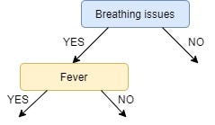
IG(Sʙʏ, Cough) = 0.09

IG of Fever is greater than that of Cough, so we select Fever as the left branch of Breathing Issues:

Our tree now looks like this:

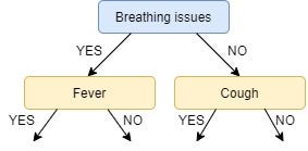
Next, we find the feature with the maximum IG for the right branch of Breathing Issues. But, since there is only one unused feature left we have no other choice but to make it the right branch of the root node.

So our tree now looks like this:

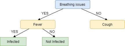
There are no more unused features, so we stop here and jump to the final step of creating the leaf nodes.

For the left leaf node of Fever, we see the subset of rows from the original data set that has Breathing Issues and Fever both values as YES.

+-------+-------+------------------+----------+
| Fever | Cough | Breathing issues | Infected |
+-------+-------+------------------+----------+
| YES   | YES   | YES              | YES      |
+-------+-------+------------------+----------+
| YES   | NO    | YES              | YES      |
+-------+-------+------------------+----------+
| YES   | YES   | YES              | YES      |
+-------+-------+------------------+----------+
| YES   | NO    | YES              | YES      |
+-------+-------+------------------+----------+
| YES   | NO    | YES              | YES      |
+-------+-------+------------------+----------+

Since all the values in the target column are YES, we label the left leaf node as YES, but to make it more logical we label it Infected.

Similarly, for the right node of Fever we see the subset of rows from the original data set that have Breathing Issues value as YES and Fever as NO.

+-------+-------+------------------+----------+
| Fever | Cough | Breathing issues | Infected |
+-------+-------+------------------+----------+
| NO    | YES   | YES              | YES      |
+-------+-------+------------------+----------+
| NO    | YES   | YES              | NO       |
+-------+-------+------------------+----------+
| NO    | YES   | YES              | NO       |
+-------+-------+------------------+----------+

Here not all but most of the values are NO, hence NO or Not Infected becomes our right leaf node.

Our tree, now, looks like this:

We repeat the same process for the node Cough, however here both left and right leaves turn out to be the same i.e. NO or Not Infected as shown below:

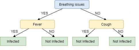
Looks Strange, doesn’t it?I know! The right node of Breathing issues is as good as just a leaf node with class ‘Not infected’. This is one of the Drawbacks of ID3, it doesn’t do pruning.

Pruning is a mechanism that reduces the size and complexity of a Decision tree by removing unnecessary nodes. More about pruning can be found here.

Another drawback of ID3 is overfitting or high variance i.e. it learns the dataset it used so well that it fails to generalize on new data.

Characteristics of ID3 Algorithm are as follows:

ID3 uses a greedy approach that's why it does not guarantee an optimal solution; it can get stuck in local optimums.

ID3 can overfit to the training data (to avoid overfitting, smaller decision trees should be preferred over larger ones).

This algorithm usually produces small trees, but it does not always produce the smallest possible tree.

ID3 is harder to use on continuous data (if the values of any given attribute is continuous, then there are many more places to split the data on this attribute, and searching for the best value to split by can be time consuming).

Learn ID3 with an example 

https://iq.opengenus.org/id3algorithm/#:~:text=ID3% %2C%20stands%20for%20Iterative,or%20minimum%20Entropy%20(H).

Video 

#Decision Tree classifier implementation in Python

import pandas as pd

df = pd.read_csv("titanic.csv")

df.head()

df.drop(['PassengerId','Name','SibSp','Parch','Ticket','Cabin','Embarked'],axis='columns',inplace=True)

df.head()

inputs = df.drop('Survived',axis='columns')

target = df.Survived

inputs.Sex = inputs.Sex.map({'male': 1, 'female': 2})

inputs.Age = inputs.Age.fillna(inputs.Age.mean())

from sklearn.model_selection import train_test_split

X_train, X_test, y_train, y_test = train_test_split(inputs,target,test_size=0.2)

from sklearn import tree

model = tree.DecisionTreeClassifier()

model.fit(X_train,y_train)

model.score(X_test,y_test)

Lean The Details Here.....Text Book Chapter