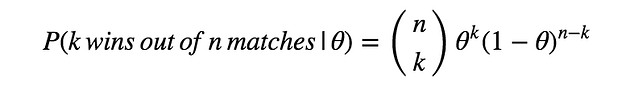
The question here is, how to calculate $P(\theta|D)$? we checked the way to calculate $P(D|\theta)$but haven’t seen the way to calculate $P(\theta|D)$. To do so, we need to use Bayes’ theorem below.


with this theorem, we can calculate the posterior probability $P(\theta|D)$ using the likelihood $P(D|\theta)$ and the prior probability $P(\theta)$.
There’s $P(D)$ in the equation, but $P(D)$ is independent to the value of $\theta$. Since we’re only interested in finding $\theta$ maximising $P(\theta|D)$, we can ignore $P(D)$ in our maximisation.
The equation above means that the maximization of the posterior probability $P(\theta|D)$ with respect to $\theta$ is equal to the maximization of the product of Likelihood $P(D|\theta)$ and Prior probability $P(\theta)$ with respect to $\theta$.
Intrinsically, we can use any formulas describing probability distribution as $P(\theta)$ to express our prior knowledge well. However, for the computational simplicity, specific probability distributions are used corresponding to the probability distribution of likelihood. It’s called conjugate prior distribution.
In this example, the likelihood $P(D|\theta)$ follows binomial distribution. Since the conjugate prior of binomial distribution is Beta distribution, we use Beta distribution to express $P(\theta)$ here. Beta distribution is described as below.


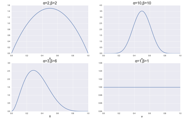
Where, α and β are called hyperparameter, which cannot be determined by data. Rather we set them subjectively to express our prior knowledge well. For example, graphs below are some visualisation of Beta distribution with different values of α and β. You can see the top left graph is the one we used in the example above (expressing that θ=0.5 is the most likely value based on the prior knowledge), and the top right graph is also expressing the same prior knowledge but this one is for the believer that past seasons’ results are reflecting Liverpool’s true capability very well.
Figure 2. Visualizations of Beta distribution with different values of α and β
A note here about the bottom right graph: when α=1 and β=1, it means we don’t have any prior knowledge about $\theta$. In this case the estimation will be completely same as the one by MLE.
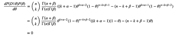
A note here about the bottom right graph: when α=1 and β=1, it means we don’t have any prior knowledge about θ. In this case the estimation will be completely same as the one by MLE.So, by now we have all the components to calculate $P(D|\theta)P(\theta)$ to maximise.
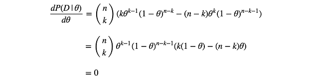
As same as MLE, we can get $\theta$ maximising this by having derivative of the this function with respect to $\theta$, and setting it to zero.
By solving this, we obtain following.


In this example, assuming we use α=10 and β=10, then $\theta=(30+10–1)/(38+10+10–2) = 39/56 = 69.6%$
Example:
Let's consider an example using a Bernoulli distribution with a known prior.
Given Data and Model
Suppose we have a set of observations from a Bernoulli process:
We want to estimate the parameter
, the probability of success. Assume we have a Beta prior for
:
where and are the parameters of the Beta distribution.
Step-by-Step Calculation
Likelihood: The likelihood of the data given is:
where is the number of successes (sum of the data) and is the total number of observations.
Prior: The prior distribution is given by the Beta distribution:
Posterior: Combining the likelihood and the prior using Bayes' theorem:
The posterior distribution is also a Beta distribution with updated parameters
and MAP Estimate: The mode of the Beta distribution (which is the MAP estimate) is given by:
This formula is valid for .
Example with Specific Values
Let's assume and for the prior. Given the data
- (total number of observations)
- (number of successes)
The posterior distribution parameters are:
So the MAP estimate for is:
********************************************************************************
More Examples
Example:
To illustrate Bayes rule, consider a medical diagnosis problem in which there are two alternative hypotheses: (1) that the patien; has a- articular form of cancer.and (2) that the patient does not. The available data is from a particular laboratory test with two possible outcomes: + (positive) and -(negative). We have prior knowledge that over the entire population of people only .008 have this disease.
Furthermore, the lab test is only an imperfect indicator of the disease. The test returns a correct positive result in only 98% of the cases in which the disease is actually present and a correct negative result in only 97% of the cases in which the disease is not present. In other cases, the test returns the opposite result. The above situation can be summarized by the following probabilities:
$P(cancer)=0.008$ $P(\neg cancer)=0.992$
$P(+|cancer)=0.98$ $P(-|cancer)=0.02$
$P(+|\neg cancer)=0.03$ $P(-|\neg cancer)=0.97$
Suppose we now observe a new patient for whom the lab test returns a positive result. Should we diagnose the patient as having cancer or not? The maximum a posteriori hypothesis can be found using Equation
$P(h|D)=P(D|h)*P(h)$
$P(cancer|+)=P(+|cancer)*P(cancer)=0.98*0.008=0.0078$
$P(\neg cancer|+)=P(+|\neg cancer)*P(\neg cancer)=0.03*0.992=0.0298$
Thus, $h_{MAP}= \neg cancer$
Example:
Suppose that X is a discrete random variable with the following probability
mass function: where $0 \le \theta \le 1$ is a parameter. The following 10 independent observations
were taken from such a distribution: (3,0,2,1,3,2,1,0,2,1). What is the maximum likelihood estimate of $\theta$.
$X \quad \quad \quad 0 \quad 1 \quad \quad 2 \quad \quad \quad 3$
$P(X) \quad \frac{2\theta}{3} \quad \frac{\theta}{3} \quad \frac{2(1 -\theta)}{3}\quad \frac{(1 - \theta)}{3}$
Since the sample is (3,0,2,1,3,2,1,0,2,1), the likelihood is
$L(\theta) = P(X = 3)P(X = 0)P(X = 2)P(X = 1)P(X = 3)P(X = 2)P(X = 1)P(X = 0)P(X = 2)P(X = 1)$
Substituting from the probability distribution given above, we have
$L(\theta)=\prod P(X_i|\theta)=\left(\frac{2\theta}{3}\right)^2\left(\frac{\theta}{3}\right)^3\left(\frac{2(1-\theta)}{3}\right)^3\left(\frac{(1-\theta)}{3}\right)^2$
Clearly, the likelihood function $L(\theta)$ is not easy to maximize.
Let us look at the log likelihood function
$l(\theta)=log L(\theta)=\sum_{i=1}^n logP(X_i,\theta)$
$\quad \quad=2(log\frac{2}{3}+\log\theta)+3(log\frac{1}{3}+\log\theta)+3(log\frac{2}{3}+\log(1-\theta))+2(log\frac{1}{3}+\log(1-\theta))$
$\quad \quad = C + 5log \theta + 5 log(1- \theta)$
where C is a constant which does not depend on $\theta$. It can be seen that the log likelihood
function is easier to maximize compared to the likelihood function.
Let the derivative of $l(\theta)$ with respect to $\theta$ be zero:
$\frac{\mathrm{d} l(\theta)}{\mathrm{d} \theta}=\frac{5}{\theta}-\frac{5}{1-\theta}=0$
and the solution gives us the MLE, which is $\theta = 0.5$.
Example.
A coin is flipped 100 times.Given that there are 55 heads, find the maximum likelihood estimate for the probability $p$ of heads on a single toss.
We can think of counting the number of heads in 100 tosses as an experiment.For a given value of $p$ , the probability of getting 55 heads in this experiment is the Binomial Probability
$P(55\quad heads)=\binom{100}{55}p^{55}(1-p)^{45}$
The probability of getting 55 heads depends on value of $p$.So lets include this as a notion of conditional probability.
$P(55\quad heads|p)=\binom{100}{55}p^{55}(1-p)^{45}$
Experiment:Flip the coin 100 times and count the number of heads.
Data:The data is the result of the experiment.In this case it is`55heads'.
Parameter(s) of interest:We are interested in the value of the unknown parameter p.
Likelihood,or likelihood function:this is $P(data|p)$:Note it is a function of both the data and the parameter $p$.
In this case the likelihood is
$P(55\quad heads|p)=\binom{100}{55}p^{55}(1-p)^{45}$
Notes:1.The likelihood $P(data|p)$ changes as the parameter of interest $p$ changes.
Definition:Given data the maximum likelihood estimate(MLE)for the parameter $p$ is the value of $p$ that maximizes the likelihood $P(data|p)$.That is,the MLE is the value of $p$ for which the data is most likely.
In order to find the maximum value we can take derivative of the MLE function,set it to zero and solve for $p$.
$\frac{\mathrm{d} }{\mathrm{d} p} P(data|p)=\binom{100}{55}(55p^{54}(1-p)^{45}-p^{55}45(1-p)^{44})=0$
$55p^{54}(1-p)^{45}=p^{55}45(1-p)^{44}$
$55(1-p)=45p$
$55=100p$
$p=55/100=0.55$
So the MLE is 0.55
Note:
1.The MLE for $p$ turned out to be exactly the fraction of heads we saw in our data.
2.The MLE is computed from the data.That is,it is a statistic.
3.Officially you should check that the critical point is indeed a maximum.You can do this with the second derivative test.
Example .Suppose that the lifetime of bulbs is modeled by an exponential distribution with(unknown)parameter $\lambda$.We test 5 bulbs and find they have lifetimes of 2,3,1,3,and 4 years,respectively.What is the MLE for $\lambda$?
The Exponential Distribution: A continuous random variable $X$ is said to have an Exponential(λ) distribution if it has probability density function $f_X(x|λ) = λe^{-λx}$ for $x > 0$ and 0 for $x ≤ 0$ , where $λ > 0$ is called the rate of the distribution.
Let $X_I$ be the life time of the $i^{th}$ bulb and let $x_i$ be the value $X_i$ takes, then each $X_i$ has a pdf $f_{X_i}(x_i)=\lambda e^{- \lambda x_i}$. We assume that life time of bulbs are independent, so the joint pdf is the product of the individual densities:
$f(x_1,x_2,x_3,x_4,x_5|\lambda)=(\lambda e^{-\lambda x_1})(\lambda e^{-\lambda x_2})(\lambda e^{-\lambda x_3})(\lambda e^{-\lambda x_4})(\lambda e^{-\lambda x_5})$
$f(x_1,x_2,x_3,x_4,x_5|\lambda)=\lambda^5 e^{-\lambda(x_1+x_2+x_3+x_4+x_5)}$
$f(2,3,1,3,4|\lambda)=\lambda^5 e^{-\lambda(2+3+1+3+4)}$
$f(2,3,1,3,4|\lambda)=\lambda^5 e^{-13\lambda}$
$ln \quad f(2,3,1,3,4|\lambda)=ln(\lambda^5)+ln( e^{-13\lambda})=5ln(\lambda)-13\lambda$
$\frac{\mathrm{d} }{\mathrm{d} \lambda}log likely hood=\frac{5}{\lambda}-13=0$
$\lambda=\frac{5}{13}$
It is noted that the MLE $\lambda=\frac{5}{13}$, which is equal to the reciprocal of sample mean($\bar{x}$)
In general the MLE of $\lambda$ is
$\lambda=\frac{n}{x_1+,x_2,\cdots+x_n}$
Example
Normal distributions
Suppose the data $x_1,x_2,\ldots x_n$is drawn from a $N(\mu,\sigma)$ distribution,where $\mu$ and $\sigma$ are unknown.Find the maximum likelihood estimate for the pair $(\mu,\sigma)$.
Let uppercase $X_1,X_2\ldots,X_n$ be i.i.d. $N(\mu;\sigma)$ random variables,and let lower case $x_i$ be the value $X_i$ takes.The density for each $X_i$ is
$f_{X_i}(x_i)=\frac{1}{\sqrt{2\pi}\sigma}e^{\frac{-(x_i-\mu)^2}{2\sigma^2}}$
Since the $X_i$ are independent their joint pdf is the product of the individual pdf's:
$f(x_1,x_2,\ldots,x_n|\mu,\sigma)=\left(\frac{1}{\sqrt{2\pi}\sigma}\right )^ne^{-\sum_{i=1}^n\frac{(x_i-\mu)^2}{2\sigma^2}}$
The log likelihood is
$ln(f(x_1,x_2,\ldots,x_n|\mu,\sigma))=-nln(\sqrt{2\pi})-nln(\sigma)-\sum_{i=1}^n\frac{(x_i-\mu)^2}{2\sigma^2}$
Since $ln(f(x_1,x_2,\ldots,x_n|\mu,\sigma))$ is a function of two variables $\mu,\sigma$, we can use partial derivatives to find MLE
$\frac{\partial }{\partial\mu}ln(f(x_1,x_2,\ldots,x_n|\mu,\sigma))=\sum_{i=1}^n\frac{(x_i-\mu)}{\sigma^2}=0$
$\sum_{i=1}^n x_i=n\mu$
$\hat\mu=\frac{\sum_{i=1}^n x_i}{n}=\bar{x}$
To find $\hat{\sigma}$ we can differentiate and solve for $\sigma$
$\frac{\partial }{\partial\sigma}ln(f(x_1,x_2,\ldots,x_n|\mu,\sigma))=-\frac{n}{\sigma}+\sum_{i=1}^n\frac{(x_i-\mu)^2}{\sigma^3}=0$
$\hat{\sigma}^2=\sum_{i=1}^n\frac{(x_i-\mu)^2}{n}$
we already know that $\mu=\bar{x}$, so we can use that value.
So the MLE are
$\hat{\mu}=\bar{x}= $ mean of the data
$\hat{\sigma^2}=\sum_{i=1}^{n}\frac{1}{n}(x-\bar{x})^2$= variance of the data
Example
MLE of the Poisson Distribution..
Poisson distribution is a probability distribution that is used to show how many times an event is likely to occur over a specified period. In other words, it is a count distribution. Poisson distributions are often used to understand independent events that occur at a constant rate within a given interval of time. It was named after French mathematician Siméon Denis Poisson.
The Poisson distribution is a discrete function, meaning that the variable can only take specific values in a (potentially infinite) list. Put differently, the variable cannot take all values in any continuous range
The probability mass function is
$f(x)=\frac{\lambda^x}{x!}e^{-\lambda}$
$x$ is the number of occurrences
where $\lambda$ is the Expected value of $x$ that is equal to its variance
The likelihood function is the product of the PMF of the observed values $x_1,x_2,\ldots,x_n$
$L(x_1,x_2,\ldots,x_n|\lambda)=\prod_{j=1}^n\frac{\lambda^{x_j}e^{-\lambda}}{x_j!}$
The log likilihood function is
$ln(L(x_1,x_2,\ldots,x_n|\lambda))=ln(\prod_{j=1}^n\frac{\lambda^{x_j}e^{-\lambda}}{x_j!})$
$=\sum_{j=1}^n ln(\lambda^{x_j})+ln(e^{-\lambda})-ln(x_j!)$
$=\sum_{j=1}^n x_j ln(\lambda)-\lambda-ln(x_j!)$
$=-n(\lambda)+ln(\lambda )\sum_{j=1}^n x_j-\sum_{j=1}^n ln(x_j!)$
Next, we can calculate the derivative of the natural log likelihood function with respect to the parameter λ:Set the derivative equal to zero and solve for λ.


Comments
Post a Comment