Neural Network and Training
Neural Networks (ANN - Artificial Neural Network)
Introduction
The term "Artificial Neural Network" is derived from Biological neural networks that develop the structure of a human brain. Similar to the human brain that has neurons interconnected to one another, artificial neural networks also have neurons that are interconnected to one another in various layers of the networks. These neurons are known as nodes.
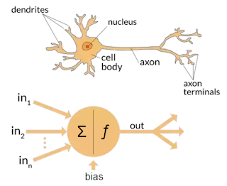
An Artificial Neural Network in the field of Artificial intelligence where it attempts to mimic the network of neurons makes up a human brain so that computers will have an option to understand things and make decisions in a human-like manner. The artificial neural network is designed by programming computers to behave simply like interconnected brain cells. There are around 1000 billion neurons in the human brain. Each neuron has an association point somewhere in the range of 1,000 and 100,000. In the human brain, data is stored in such a manner as to be distributed, and we can extract more than one piece of this data when necessary from our memory parallelly. We can say that the human brain is made up of incredibly amazing parallel processors.

A biological neuron in comparison to an artificial neural network: (a) human neuron; (b) artificial neuron; (c) biological synapse; and (d) ANN synapses
Perceptrons
ANN system is based on a unit called a perceptron. It was invented in the late 1950s by Frank Rosenblatt.A perceptron takes a vector of real-valued inputs, calculates a linear combination of these inputs, then outputs a 1 if the result is greater than some threshold and -1 otherwise.

More precisely, given inputs $x_l$ through $x_n$, the output $o(x_1, . . . , x_n)$ computed by the perceptron is
1& if w_0+w_1x_1+\cdots+w_nx_n > 0\\
-1& otherwise
\end{matrix}\right.$
where each $w_i$ is a real-valued constant, or weight, that determines the contribution of input $x_i$ to the perceptron output. Notice the quantity $ (-w_0)$ is a threshold that the weighted combination of inputs $w_lx_l + \ldots + w_nx_n$ must surpass in order for the perceptron to output a 1.
To simplify notation, we imagine an additional constant input $x_0 = 1$, allowing us to write the above inequality as $\sum_{i=0}^n w_ix_i > 0$, or in vector form as $w_ix_i > 0$. For brevity, we will sometimes write the perceptron function as
$o(\vec{x})=sgn(\vec{w}.\vec{x})$
where
$sgn(y)=\left\{\begin{matrix}1& if y> 0\\-1& otherwise
\end{matrix}\right.$
Learning a perceptron involves choosing values for the weights $w_0, . . . , w_n$.Therefore, the space $H$ of candidate hypotheses considered in perceptron learning is the set of all possible real-valued weight vectors
$H=\{\vec{w}| \vec{w} \in \mathbb{R}^{n+1}\}$Representational Power of Perceptrons
We can view the perceptron as representing a hyperplane decision surface in the n-dimensional space of instances (i.e., points). The perceptron outputs a 1 for instances lying on one side of the hyperplane and outputs a -1 for instances lying on the other side, as illustrated in Figure below. The equation for this decision hyperplane is $\vec{w}.\vec{x} = 0$. Of course, some sets of positive and negative examples cannot be separated by any hyperplane. Those that can be separated are called linearly separable sets of examples.

A single perceptron can be used to represent many boolean functions. For example, if we assume boolean values of 1 (true) and -1 (false), then one way to use a two-input perceptron to implement the AND function is to set the weights $w_0 = -0.8$, and $w_2 = w_3 = .5$. This perceptron can be made to represent the OR function instead by altering the threshold to $w_0= -.3$. In fact, AND and OR can be viewed as special cases of m-of-n functions: that is, functions where at least $m$ of the $n$ inputs to the perceptron must be true. The OR function corresponds to $m= 1$ and the AND function to $m = n$. Any m-of-n function is easily represented using a perceptron by setting all input weights to the same value (e.g., 0.5) and then setting the threshold $w_0$ accordingly. Perceptrons can represent all of the primitive boolean functions AND, OR,NAND ($\neg$ AND), and NOR ($\neg$ OR). Unfortunately, however, some boolean functions cannot be represented by a single perceptron, such as the XOR function whose value is 1 if and only if $x_l \ne x_2$. Note the set of linearly nonseparable training examples shown in Figure (b) corresponds to this XOR function.
The ability of perceptrons to represent AND, OR, NAND, and NOR is important because every boolean function can be represented by some network of interconnected units based on these primitives. In fact, every boolean function can be represented by some network of perceptrons only two levels deep, in which the inputs are fed to multiple units, and the outputs of these units are then input to a second, final stage. One way is to represent the boolean function in disjunctive normal form (i.e., as the disjunction (OR) of a set of conjunctions (ANDs) of the inputs and their negations). Note that the input to an AND perceptron can be negated simply by changing the sign of the corresponding input weight.Because networks of threshold units can represent a rich variety of functions and because single units alone cannot, we will generally be interested in learning multilayer networks of threshold units.
XOR Problem
This problem is not linearly seperable. However the XOR operation can be represented as
$A \bigoplus B= A \bar{B} + \bar{A} B=(A+B)(\bar{A} + \bar{B})=(A+B).(\bar{AB})$
We can train the model for OR and NAND data
we are performing a logical AND on the outputs of two logic gates (where the first one is an OR and the second one a NAND) and that both functions are being passed the same input ($x_1$ and $x_2$).

What we now have is a model that mimics the XOR function.

If we plot the decision boundaries from our model, — which is basically an AND of our OR and NAND models — we get something like this:

Out of all the 2 input logic gates, the XOR and XNOR gates are the only ones that are not linearly-separable.
Though our model works, it doesn’t seem like a viable solution to most non-linear classification or regression tasks. It’s really specific to this case, and most problems can’t be split into just simple intermediate problems that can be individually solved and then combined.
A potential decision boundary could be something like this:
The Multi-layered Perceptron can solve this problem.The overall components of a MLP like input and output nodes, activation function and weights and biases are the same as those we just discussed in a perceptron.The biggest difference is that a MLP can have hidden layers.
An MLP is generally restricted to having a single hidden layer.
The hidden layer allows for non-linearity. A node in the hidden layer isn’t too different to an output node: nodes in the previous layers connect to it with their own weights and biases, and an output is computed, generally with an activation function.
Perceptron Training Rule
Although we are interested in learning networks of many interconnected units, let us begin by understanding how to learn the weights for a single perceptron. Here the precise learning problem is to determine a weight vector that causes the perceptron to produce the correct $\pm1$ output for each of the given training examples.
Several algorithms are known to solve this learning problem. Here we consider two: the perceptron rule and the delta rule. These two algorithms are guaranteed to converge to somewhat different acceptable hypotheses, under somewhat different conditions. They are important to ANNs because they provide the basis for learning networks of many units.
One way to learn an acceptable weight vector is to begin with random weights, then iteratively apply the perceptron to each training example, modifying the perceptron weights whenever it misclassifies an example. This process is repeated, iterating through the training examples as many times as needed until the perceptron classifies all training examples correctly. Weights are modified at each step according to the perceptron training rule, which revises the weight $w_i$ associated with input $x_i$ according to the rule
$w_i=w_i+ \Delta w_i$
where
$\Delta w_i=\eta(t-o)x_i$
Here $t$ is the target output for the current training example, $o$ is the output generated by the perceptron, and $\eta$ is a positive constant called the learning rate. The role of the learning rate is to moderate the degree to which weights are changed at each step. It is usually set to some small value (e.g., 0.1) and is sometimes made to decay as the number of weight-tuning iterations increases.
Why should this update rule converge toward successful weight values? To get an intuitive feel, consider some specific cases. Suppose the training example is correctly classified already by the perceptron. In this case, $(t - o)$ is zero, making $\Delta w_i$ zero, so that no weights are updated. Suppose the perceptron outputs a -1,when the target output is + 1. To make the perceptron output a + 1 instead of - 1 in this case, the weights must be altered to increase the value of $\vec{w_i}\vec{x_i}$. For example, if $x_i \gt 0$, then increasing $w_i$ will bring the perceptron closer to correctly classifying this example. Notice the training rule will increase $w_i$, in this case, because $\eta,(t - o)$, and $x_i$ are all positive.
For example, if $x_i = .8, \eta = 0.1, t = 1,$ and $o = - 1$,then the weight update will be $\Delta w_i = \eta(t - o)x_i = 0.1(1 - (-1))0.8 = 0.16.$
On the other hand, if $t = -1$ and $o= 1$, then weights associated with positive $x_i$ will be decreased rather than increased.
In fact, the above learning procedure can be proven to converge within a finite number of applications of the perceptron training rule to a weight vector that correctly classifies all training examples, provided the training examples are linearly separable and provided a sufficiently small $\eta$ is used. If the data are not linearly separable, convergence is not assured.
Gradient Descent and the Delta Rule
Although the perceptron rule finds a successful weight vector when the training examples are linearly separable, it can fail to converge if the examples are not linearly separable. A second training rule, called the delta rule, is designed to overcome this difficulty. If the training examples are not linearly separable, the delta rule converges toward a best-fit approximation to the target concept.
The key idea behind the delta rule is to use gradient descent to search the hypothesis space of possible weight vectors to find the weights that best fit the training examples. This rule is important because gradient descent provides the basis for the BACKPROPAGATION algoritm, which can learn networks with many interconnected units. It is also important because gradient descent can serve as the basis for learning algorithms that must search through hypothesis spaces containing many different types of continuously parameterized hypotheses.
The delta training rule is best understood by considering the task of training an unthresholded perceptron; that is, a linear unit for which the output $o$ is given by
$o(\vec{x})=\vec{w}.\vec{x}$
Thus, a linear unit corresponds to the first stage of a perceptron, without the threshold.
In order to derive a weight learning rule for linear units, let us begin by specifying a measure for the training error of a hypothesis (weight vector), relative to the training examples. Although there are many ways to define this error, one common measure that will turn out to be especially convenient is
$E(\vec{w})=\frac{1}{2}\sum_{d \in D} (t_d-o_d)^2$
Gradient descent search determines a weight vector that minimizes $E$ by starting with an arbitrary initial weight vector, then repeatedly modifying it in small steps. At each step, the weight vector is altered in the direction that produces the steepest descent along the error surface. This process continues until the global minimum error is reached.
How can we calculate the direction of the steepest descent.This direction can be found by computing the derivative of $E$ with respect to each component of the vector $\vec{w}$. This vector derivative is called the gradient of $E$ with respect to $\vec{w}$, written as $\nabla E(\vec{w})$
\end{bmatrix}$
When interpreted as a vector in weight space, the gradient specijies the direction that produces the steepest increase in $E$. The negative of this vector therefore gives the direction of steepest decrease.
Since the gradient specifies the direction of steepest increase of $E$, the training rule for gradient descent is
$\vec{w}=\vec{w}+\Delta \vec{w}$
where
$\Delta w_i= - \eta \frac{\partial E}{\partial w_i}$
which makes it clear that steepest descent is achieved by altering each component $w_i$, of $\vec{w}$ in proportion to $\frac{\partial E}{\partial w_i}$
To construct a practical algorithm for iteratively updating weights according to above equation, we need an efficient way of calculating the gradient at each step. Fortunately, this is not difficult. The vector of $\frac{\partial E}{\partial w_i}$ derivatives that form the gradient can be obtained by differentiating $E$ from Equation as
$\frac{\partial E}{\partial w_i} =\sum_{d \in D} (t_d-o_d).(-x_{id})$
where $x_{id}$ denotes the single input component $x_i$ for training example $d$. We now have an equation that gives in terms of the linear unit inputs $x_{id}$, outputs $o_d$, and target values $t_d$ associated with the training examples.
Substituting this in the weight update rule of gradient descent gives
$\Delta w_i= \eta \sum_{d \in D} ( t_d-o_d)x_{id}------(A)$To summarize, the gradient descent algorithm for training linear units is as follows:
Pick an initial random weight vector.
Apply the linear unit to all training examples, then compute $\nabla w_i$ for each weight according to above equation .
Update each weight $w_i$ by adding $\nabla w_i$, then repeat this process.

Because the error surface contains only a single global minimum,this algorithm will converge to a weight vector with minimum error, regardless of whether the training examples are linearly separable, given a sufficiently small learning rate $\eta$ is used. If $\eta$ is too large, the gradient descent search runs the risk of overstepping the minimum in the error surface rather than settling into it. For this reason, one common modification to the algorithm is to gradually reduce the value of $\eta$ as the number of gradient descent steps grows.
Stochastic Approximation To Gradient Descent
Gradient descent is an important general paradigm for learning. It is a strategy for searching through a large or infinite hypothesis space that can be applied whenever
(1) the hypothesis space contains continuously parameterized hypotheses (e.g., the weights in a linear unit), and
(2) the error can be differentiated with respect to these hypothesis parameters.
The key practical difficulties in applying gradient descent are
(1) converging to a local minimum can sometimes be quite slow (i.e.,it can require many thousands of gradient descent steps), and
(2) if there are multiple local minima in the error surface, then there is no guarantee that the procedure will find the global minimum.
One common variation on gradient descent intended to alleviate these difficulties is called incremental gradient descent, or alternatively stochastic gradient descent. Whereas the gradient descent training rule presented in Equation (A) computes weight updates after summing over all the training examples in $D$, the idea behind stochastic gradient descent is to approximate this gradient descent search by updating weights incrementally, following the calculation of the error for each individual example. The modified training rule is like the training rule given by Equation (A) except that as we iterate through each training example we update the weight according to
$\Delta w_i= \eta ( t-o) x_i ----------(B)$
where $t, o$, and $x_i$ are the target value, unit output, and ith input for the training example in question.To modify the gradient descent algorithm to implement this stochastic approximation, Equation (T4.2) is simply deleted and Equation (T4.1) replaced by $ w_i =w_i + \eta (t - o) x_i$. One way to view this stochastic gradient descent is to consider a distinct error function $E_d(\vec{w})$ defined for each individual training example $d$ as follows
$E_d(\vec{w})=\frac{1}{2}(t_d-o_d)^2$
where $t$, and $o$ are the target value and the unit output value for training example $d$. Stochastic gradient descent iterates over the training examples $d$ in $D$,at each iteration altering the weights according to the gradient with respect to $E_d(\vec{w})$. The sequence of these weight updates, when iterated over all training examples, provides a reasonable approximation to descending the gradient with
respect to our original error function $E(\vec{w})$. By making the value of $\eta$ (the gradient descent step size) sufficiently small, stochastic gradient descent can be made to approximate true gradient descent arbitrarily closely. The key differences between standard gradient descent and stochastic gradient descent are:
- In standard gradient descent, the error is summed over all examples before updating weights, whereas in stochastic gradient descent weights are updated upon examining each training example.
- Summing over multiple examples in standard gradient descent requires more computation per weight update step. On the other hand, because it uses the true gradient, standard gradient descent is often used with a larger step size per weight update than stochastic gradient descent.
- In cases where there are multiple local minima with respect to $E(\vec{w})$ ,stochastic gradient descent can sometimes avoid falling into these local minima because it uses the various $\nabla E_d(\vec{w})$ rather than $\nabla E(\vec{w})$ to guide its search.
Both stochastic and standard gradient descent methods are commonly used in practice.The training rule in Equation (B) is known as the delta rule, or sometimes the LMS (least-mean-square) rule, Adaline rule, or Widrow-Hoff rule (after its inventors). Notice the delta rule in Equation (B) is similar to the perceptron training rule . In fact, the two expressions appear to be identical. However, the rules are different because in the delta rule $o$ refers to the linear unit output $o(\vec{x}) =\vec{w}.\vec{x}$ whereas for the perceptron rule $o$ refers to the thresholded output $o(\vec{x}) = sgn(\vec{w}.\vec{x}).$
We have considered two similar algorithms for iteratively learning perceptron weights. The key difference between these algorithms is that the perceptron training rule updates weights based on the error in the thresholded perceptron output,whereas the delta rule updates weights based on the error in the unthresholded linear combination of inputs.
The difference between these two training rules is reflected in different convergence properties. The perceptron training rule converges after a finite number of iterations to a hypothesis that perfectly classifies the training data, provided the training examples are linearly separable. The delta rule converges only asymptotically toward the minimum error hypothesis, possibly requiring unbounded time, but converges regardless of whether the training data are linearly separable.
A third possible algorithm for learning the weight vector is linear programming.Linear programming is a general, efficient method for solving sets of linear inequalities. Notice each training example corresponds to an inequality of the form $\vec{w}.\vec{x} > 0$ or $\vec{w}.\vec{x} \le 0$, and their solution is the desired weight vector. Unfortunately,this approach yields a solution only when the training examples are linearly separable; however, Duda and Hart (1973, p. 168) suggest a more subtle formulation that accommodates the nonseparable case. In any case, the approach of linear programming does not scale to training multilayer networks, which is our primary concern. In contrast, the gradient descent approach, on which the delta rule is based, can be easily extended to multilayer networks.
As noted in previous section, single perceptrons can only express linear decision surfaces. In contrast, the kind of multilayer networks learned by the BACKPROPAGATION algorithm are capable of expressing a rich variety of nonlinear decision surfaces.
What type of unit shall we use as the basis for constructing multilayer networks?At first we might be tempted to choose the linear units discussed in the previous section for which we have already derived a gradient descent learning rule. However, multiple layers of cascaded linear units still produce only linear functions,and we prefer networks capable of representing highly nonlinear functions. The perceptron unit is another possible choice, but its discontinuous threshold makes it undifferentiable and hence unsuitable for gradient descent. What we need is a unit whose output is a nonlinear function of its inputs, but whose output is also a differentiable function of its inputs. One solution is the sigmoid unit-a unit very much like a perceptron, but based on a smoothed, differentiable threshold function.
The sigmoid unit is illustrated in Figure. Like the perceptron, the sigmoid unit first computes a linear combination of its inputs, then applies a threshold to the result. In the case of the sigmoid unit, however, the threshold output is a continuous function of its input.

$\sigma(y)=\frac{1}{1+e^{-y}}$
$\sigma$ is often called the sigmoid function or, alternatively, the logistic function. Note its output ranges between 0 and 1, increasing monotonically with its input .Because it maps a very large input domain to a small range of outputs, it is often referred to as the squashing function of the unit. The sigmoid function has the useful property that its derivative is easily expressed in terms of its output
$\frac{\mathrm{d} \sigma(y)}{\mathrm{d} y}=\sigma(y)(1-\sigma(y))$
As we shall see, the gradient descent learning rule makes use of this derivative.Other differentiable functions with easily calculated derivatives are sometimes used in place of $\sigma$. For example, the term $e^{-y}$ in the sigmoid function definition is sometimes replaced by $e^{-ky}$ where $k$ is some positive constant that determines the steepness of the threshold. The function $tanh$ is also sometimes used in place of the sigmoid function
The Back propagation Algorithm
The BACKPROPAGATION Algorithm learns the weights for a multilayer network, given a network with a fixed set of units and interconnections. It employs gradient descent to attempt to minimize the squared error between the network output values and the target values for these outputs.
Because we are considering networks with multiple output units rather than single units as before, we begin by redefining $E$ to sum the errors over all of the network output units
where $outputs$ is the set of output units in the network, and $t_{kd}$ and $o_{kd}$ are the target and output values associated with the $k$th output unit and training example $d$.
One major difference in the case of multilayer networks is that the error surface can have multiple local minima, in contrast to the single-minimum parabolic error surface Unfortunately, this means that gradient descent is guaranteed only to converge toward some local minimum, and not necessarily the global minimum error. Despite this obstacle, in practice BACKPROPAGATION has been found to produce excellent results in many real-world applications.
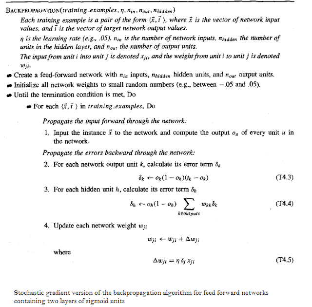
The BACKPROPAGATION Algorithm described here applies to layered feed forward networks containing two layers of sigmoid units, with units at each layer connected to all units from the preceding
layer. This is the incremental, or stochastic, gradient descent version of BACKPROPAGATION.The notation used here is the same as that used in earlier sections, with the following extensions:
$x_{ji}$ denotes the input from node $i$ to unit $j$, and $w_{ji}$ denotes the corresponding weight.
$\delta_n$, denotes the error term associated with unit $n$. It plays a role analogous to the quantity $(t - o)$ in our earlier discussion of the delta training rule. As we shall see later, $\delta_n=-\frac{\partial E}{\partial net_n}$
Notice the algorithm begins by constructing a network with the desired number of hidden and output units and initializing all network weights to small random values. Given this fixed network structure, the main loop of the algorithm then repeatedly iterates over the training examples. For each training example, it applies the network to the example, calculates the error of the network output for this example, computes the gradient with respect to the error on this example, then updates all weights in the network. This gradient descent step is iterated (often thousands of times, using the same training examples multiple times) until the network performs acceptably well.
The gradient descent weight-update rule is similar to the delta training rule. Like the delta rule, it updates each weight in proportion to the learning rate $\eta$, the input value $x_{ji}$ to which the weight is applied, and the error in the output of the unit. The only difference is that the error (t - o) in the delta rule is replaced by a more complex error term, $\delta_j$. To understand it intuitively, first consider how $\delta_k$ is computed for each network output unit $k$.$\delta_k$ is simply the familiar $(t_k - o_k)$ from the delta rule, multiplied by the factor $o_k(1 - o_k)$, which is the derivative of the sigmoid squashing function.
The $\delta_h$ value for each hidden unit $h$ has a similar form However, since training examples provide target values $t_k$ only for network outputs, no target values are directly available to indicate the error of hidden units' values. Instead, the error term for hidden unit $h$ is calculated by summing the error terms $\delta_k$ for each output unit influenced by $h$, weighting each of the $\delta_k$'s by $w_{kh}$, the weight from hidden unit $h$ to output unit $k$. This weight characterizes the degree to which hidden unit $h$ is "responsible for" the error in output unit $k$.
The algorithm updates weights incrementally, following the presentation of each training example. This corresponds to a stochastic approximation to gradient descent. To obtain the true gradient of $E$ one would sum the $\delta_j x_{ji}$ values over all training examples before altering weight values.
The weight-update loop in BACKPROPAGATION may be iterated thousands of times in a typical application. A variety of termination conditions can be used to halt the procedure. One may choose to halt after a fixed number of iterations through the loop, or once the error on the training examples falls below some threshold, or once the error on a separate validation set of examples meets some criterion. The choice of termination criterion is an important one, because too few iterations can fail to reduce error sufficiently, and too many can lead to overfitting the training data.
Adding Momentum
Because BACKPROPAGATION is such a widely used algorithm, many variations have been developed. Perhaps the most common is to alter the weight-update rule in Equation (T4.5) in the algorithm by making the weight update on the $n$th iteration depend partially on the update that occurred during the $(n - 1)$th iteration, as follows:
$\Delta w_{ji}(n)=\eta \delta_j x_{ji}+\alpha \Delta w_{ji}(n-1)$
Here $\Delta w_{ji}(n)$ is the weight update performed during the $n$th iteration through the main loop of the algorithm, and $0 \le \alpha \lt 1$ is a constant called the momentum.
Notice the first term on the right of this equation is just the weight-update rule of Equation (T4.5) in the BACKPROPAGATION Algorithm. The second term on the right is new and is called the momentum term. To see the effect of this momentum term, consider that the gradient descent search trajectory is analogous to that of a (momentum less) ball rolling down the error surface. The effect of $\alpha$ is to add momentum that tends to keep the ball rolling in the same direction from one iteration to the next. This can sometimes have the effect of keeping the ball rolling through small local minima in the error surface, or along flat regions in the surface where the ball would stop if there were no momentum. It also has the effect of gradually increasing the step size of the search in regions where the gradient is unchanging, thereby speeding convergence.
Deriving the Back propagation rule
The stochastic gradient descent involves iterating through the training examples one at a time, for each training example $d$ descending the gradient of the error $E_d$ with respect to this single example. In other words, for each training example $d$ every weight $w_{ji}$ is updated by adding to it $\Delta w_{ji}$
$\Delta w_{ji}= - \eta \frac{\partial Ed}{\partial w_{ji}}-----(C)$
where $E_d$ is the error on training example $d$, summed over all output units in the network
$E_d(\vec{w})\equiv \frac{1}{2}\sum_{k \in outputs}(t_k- o_k) ^2$Here outputs is the set of output units in the network, $t_k$ is the target value of unit $k$ for training example $d$, and $o_k$ is the output of unit $k$ given training example $d$.The derivation of the stochastic gradient descent rule is conceptually straightforward,but requires keeping track of a number of subscripts and variables.
$x_{ji}=$ The $i$th input to unit $j$
$w_{ji} =$ the weight associated with the $i$th input to unit $j$
$net_j = \sum_i w_{ji}x_{ji}$ (the weighted sum of inputs for unit $j$ )
$o_j = $ the output computed by unit $j$
$t_j=$ the target output for unit $j$
$\sigma =$ the sigmoid function
$outputs =$ the set of units in the final layer of the network
$Downstream(j)$ = the set of units whose immediate inputs include the output of unit $j$
We now derive an expression for $\frac{\partial E_d}{\partial w_{ji}}$ in order to implement the stochastic gradient descent rule seen in Equation (C). To begin, notice that weight $w_{ji}$ can influence the rest of the network only through $net_j$. Therefore, we can use the chain rule to write
$\frac{\partial E_d}{\partial w_{ji}}=\frac{\partial E_d}{\partial net_j} x_{ji}$
our remaining task is to derive a convenient expression for $\frac{\partial E_d}{\partial net_j}$.We consider two cases in turn: the case where unit $j$ is an output unit for the network, and the case where $j$ is an internal unit.
Case 1: Training Rule for Output Unit Weights
Just as $w_{ji}$ can influence the rest of the network only through $net_j$, $net_j$ can influence the network only through $o_j$. Therefore, we can invoke the chain rule again to write
$\frac{\partial E_d}{\partial net_j}=\frac{\partial E_d}{\partial o_j} \frac{\partial o_j}{\partial net_j}$
$\frac{\partial E_d}{\partial o_j}=\frac{\partial }{\partial o_j}\frac{1}{2} \sum _{k \in outputs}(t_k-o_k)^2$
The derivatives $\frac{\partial }{\partial o_j}(t_k-o_k)^2$ will be zero for all output units $k$ except when $k = j$.We therefore drop the summation over output units and simply set $k = j$.
$\frac{\partial E_d}{\partial o_j}=\frac{\partial }{\partial o_j}\frac{1}{2}(t_j-o_j)^2$
$=\frac{1}{2}2(t_j-o_j)\frac{\partial }{\partial o_j}(t_j-o_j)$
$=-(t_j-o_j)-----(1)$
Next consider the term $\frac{\partial o_j}{\partial net_j}$. Since $o_j=\sigma(net_j)$, the derivative
$\frac{\partial o_j}{\partial net_j}$ is just the derivative of the sigmoid function, which we have already noted is equal to $\sigma(net_j)(1-\sigma(net_j))$
$\frac{\partial o_j}{\partial net_j}=o_j(1-o_j)----(2)$
Combining (1) and (2) will give
$\frac{\partial E_d}{\partial net_j}=\frac{\partial E_d}{\partial o_j} \frac{\partial o_j}{\partial net_j}$
$\frac{\partial E_d}{\partial net_j}= -(t_j-o_j)o_j(1-o_j)$and combining this , we have the stochastic gradient descent rule for output units
$\Delta w_{ji}=- \eta \frac{\partial E_d}{\partial w_{ji}}=\eta (t_j-o_j)o_j(1-o_j)x_{ji}$Note this training rule is exactly the weight update rule implemented by Equations (T4.3) and (T4.5) in the algorithm
Case 2: Training Rule for Hidden Unit Weights.
In the case where $j$ is an internal, or hidden unit in the network, the derivation of the training rule for $w_{ji}$ must take into account the indirect ways in which $w_{ji}$ can influence the network outputs and hence $E_d$. For this reason, we will find it useful to refer to the set of all units immediately downstream of unit $j$ in the network (i.e., all units whose direct inputs include the output of unit $j$). We denote this set of units by $Downstream( j)$. Notice that $net_j$ can influence the network outputs (and therefore $E_d$) only through the units in $Downstream(j)$. Therefore, we can write
$=\sum_{k \in Downstream(j)}-\delta_k \quad\frac{\partial net_k}{\partial net_j}$
$=\sum_{k \in Downstream(j)}\delta_k \quad\frac{\partial net_k}{\partial o_j}\frac{\partial o_j}{\partial net_j}$
$=\sum_{k \in Downstream(j)}\delta_k \quad w_{kj}\quad \frac{\partial o_j}{\partial net_j}$$=\sum_{k \in Downstream(j)}\delta_k \quad w_{kj}\quad o_j(1-o_j)$
Rearranging terms and using $\delta_j$ to denote $-\frac{\partial E_d}{\partial net_j}$, we have
$\delta_j=o_j(1-o_j) \sum_{k \in Downstream(j)}\delta_k \quad w_{kj}$
and
$\Delta w_{ji}= \eta \delta_j x_{ji}$
How do artificial neural networks work
Artificial Neural Network can be best represented as a weighted directed graph, where the artificial neurons form the nodes. The association between the neurons outputs and neuron inputs can be viewed as the directed edges with weights. The Artificial Neural Network receives the input signal from the external source in the form of a pattern and image in the form of a vector. These inputs are then mathematically assigned by the notations $x(n)$ for every $n$ number of inputs.

Input Layer:
As the name suggests, it accepts inputs in several different formats provided by the programmer.
Hidden Layer:
The hidden layer presents in-between input and output layers. It performs all the calculations to find
hidden features and patterns.
Output Layer:
The input goes through a series of transformations using the hidden layer, which finally results in output
that is conveyed using this layer.
The artificial neural network takes input and computes the weighted sum of the inputs and includes a bias. This computation is represented in the form of a transfer function.
$\sum_{i=1}^n w_i x_i + b $
It determines weighted total and is passed as an input to an activation function to produce the output. Activation functions choose whether a node should fire or not. Only those who are fired make it to the output layer. There are distinctive activation functions available that can be applied upon the sort of task we are performing.
Afterward, each of the input is multiplied by its corresponding weights ( these weights are the details utilized by the artificial neural networks to solve a specific problem ). In general terms, these weights normally represent the strength of the interconnection between neurons inside the artificial neural network. All the weighted inputs are summarized inside the computing unit.
If the weighted sum is equal to zero, then bias is added to make the output non-zero or something else to scale up to the system's response. Bias has the same input, and weight equals to 1. Here the total of weighted inputs can be in the range of 0 to positive infinity. Here, to keep the response in the limits of the desired value, a certain maximum value is bench marked, and the total of weighted inputs is passed through the activation function.The activation function refers to the set of transfer functions used to achieve the desired output. There is a different kind of the activation function, but primarily either linear or non-linear sets of functions. Some of the commonly used sets of activation functions are the linear, Tan hyperbolic, sigmoidal and ReLu activation functions. Activation functions should be differentiable, so that a network’s parameters can be updated using back propagation.
Activation Functions
The activation function defines the output of a neuron / node given an input or set of input (output of multiple neurons). It's the mimic of the stimulation of a biological neuron.Activation function decides, whether a neuron should be activated or not by calculating weighted sum and further adding bias with it. The purpose of the activation function is to introduce non-linearity into the output of a neuron.
We know, neural network has neurons that work in correspondence of weight, bias and their respective activation function. In a neural network, we would update the weights and biases of the neurons on the basis of the error at the output. This process is known as back-propagation. Activation functions make the back-propagation possible since the gradients are supplied along with the error to update the weights and biases.
The Activation Functions can be basically divided into 2 types-
- Linear Activation Function
- Non-linear Activation Function
Linear Activation Functions
- Equation : Linear function has the equation similar to as of a straight line i.e. $y = ax$
- No matter how many layers we have, if all are linear in nature, the final activation function of last layer is nothing but just a linear function of the input of first layer.
- Range : -inf to +inf
- Uses : Linear activation function is used at just one place i.e. output layer.
- Issues : If we will differentiate linear function to bring non-linearity, result will no more depend on input “x” and function will become constant, it won’t introduce any ground-breaking behavior to our algorithm.

Pros
- It gives a range of activations, so it is not binary activation.
- We can definitely connect a few neurons together and if more than 1 fires, we could take the max ( or softmax) and decide based on that.
- For this function, derivative is a constant. That means, the gradient has no relationship with X.
- It is a constant gradient and the descent is going to be on constant gradient.
- If there is an error in prediction, the changes made by back propagation is constant and not depending on the change in input delta(x) !
For example : Calculation of price of a house is a regression problem. House price may have any big/small value, so we can apply linear activation at output layer. Even in this case neural net must have any non-linear function at hidden layers.
Non-linear Activation Function
The Nonlinear Activation Functions are the most used activation functions.It makes it easy for the model to generalize or adapt with variety of data and to differentiate between the output.
The main terminologies needed to understand for nonlinear functions are:
Derivative or Differential: Change in y-axis w.r.t. change in x-axis.It is also known as slope.
Monotonic function: A function which is either entirely non-increasing or non-decreasing.
The Nonlinear Activation Functions are mainly divided on the basis of their range or curves
1. Sigmoid or Logistic Activation Function
The Sigmoid Function curve looks like a S-shape.

The main reason why we use sigmoid function is because it exists between (0 to 1). Therefore, it is especially used for models where we have to predict the probability as an output.Since probability of anything exists only between the range of 0 and 1, sigmoid is the right choice.
The function is differentiable.That means, we can find the slope of the sigmoid curve at any two points.
The function is monotonic but function’s derivative is not.
The logistic sigmoid function can cause a neural network to get stuck at the training time.
- Equation :
- Value Range : 0 to 1
- Uses : Usually used in output layer of a binary classification, where result is either 0 or 1, as value for sigmoid function lies between 0 and 1 only so, result can be predicted easily to be 1 if value is greater than 0.5 and 0 otherwise.

Pros
- It is nonlinear in nature. Combinations of this function are also nonlinear!
- It will give an analog activation unlike step function.
- It has a smooth gradient too.
- It’s good for a classifier.
- The output of the activation function is always going to be in range (0,1) compared to (-inf, inf) of linear function. So we have our activations bound in a range. Nice, it won’t blow up the activations then.
- Towards either end of the sigmoid function, the Y values tend to respond very less to changes in X.
- It gives rise to a problem of “vanishing gradients”.
- Its output isn’t zero centered. It makes the gradient updates go too far in different directions. 0 < output < 1, and it makes optimization harder.
- Sigmoids saturate and kill gradients.
- The network refuses to learn further or is drastically slow ( depending on use case and until gradient /computation gets hit by floating point value limits ).
- The softmax function is a more generalized logistic activation function which is used for multiclass classification.
2. Softmax Function :- The softmax function is also a type of sigmoid function but is handy when we are trying to handle classification problems.
Nature :- non-linear
Uses :- Usually used when trying to handle multiple classes. The softmax function would squeeze the outputs for each class between 0 and 1 and would also divide by the sum of the outputs.
Output:- The softmax function is ideally used in the output layer of the classifier where we are actually trying to attain the probabilities to define the class of each input.
Softmax is an activation function that scales numbers/logits into probabilities. The output of a Softmax is a vector (say $v$) with probabilities of each possible outcome. The probabilities in vector $v$ sums to one for all possible outcomes or classes.
Mathematically, Softmax is defined as,
$S(y)_i=\frac{exp(y_i)}{\sum_{j=1}^n exp(y_j)}$
$n$- is the number of classes ( possible outcomes)
$y_i$ is the input
$exp(y_i)$ is the standard exponential function applied on $y_i$, the result is a smaller value closer to zero when $y_i <0$ and large value when $y_i >0$
3. Tanh or Hyperbolic Tangent Activation Function
tanh is also like logistic sigmoid but better. The range of the tanh function is from (-1 to 1). tanh is also sigmoidal (s - shaped).Tanh function also knows as Tangent Hyperbolic function. It’s actually mathematically shifted version of the sigmoid function. Both are similar and can be derived from each other.
Tanh squashes a real-valued number to the range [-1, 1]. It’s non-linear. But unlike Sigmoid, its output is zero-centered. Therefore, in practice the tanh non-linearity is always preferred to the sigmoid nonlinearity.

The function is differentiable.
The function is monotonic while its derivative is not monotonic.
The tanh function is mainly used classification between two classes.
Both tanh and logistic sigmoid activation functions are used in feed-forward nets.
Equation :-
$f(x) = tanh(x) = \frac{2}{(1 + e^{-2x})} - 1$ OR $tanh(x) = 2 * sigmoid(2x) - 1$
Value Range : -1 to +1
Nature :- non-linear

Pros
Value Range : -1 to +1
Nature :- non-linear
Uses :- Usually used in hidden layers of a neural network as it’s values lies between -1 to 1 hence the mean for the hidden layer comes out be 0 or very close to it, hence helps in centering the data by bringing mean close to 0. This makes learning for the next layer much easier.

Pros
The gradient is stronger for tanh than sigmoid ( derivatives are steeper).
Cons
Cons
Tanh also has the vanishing gradient problem.
4. ReLU (Rectified Linear Unit) Activation Function
A recent invention which stands for Rectified Linear Units. The formula is deceptively simple: $max(0,z)$ Despite its name and appearance, it’s not linear and provides the same benefits as Sigmoid (i.e. the ability to learn nonlinear functions), but with better performance. it is used in almost all the convolutional neural networks or deep learning

As you can see, the ReLU is half rectified (from bottom). $R(z)$ is zero when $z$ is less than zero and $R(z)$ is equal to $z$ when $z$ is above or equal to zero.
Range: [ 0 to infinity)
The function and its derivative both are monotonic.
But the issue is that all the negative values become zero immediately which decreases the ability of the model to fit or train from the data properly. That means any negative input given to the ReLU activation function turns the value into zero immediately in the graph, which in turns affects the resulting graph by not mapping the negative values appropriately.
Value Range :- $[0, \inf)$
Nature :- non-linear, which means we can easily backpropagate the errors and have multiple layers of neurons being activated by the ReLU function.
Uses :- ReLu is less computationally expensive than tanh and sigmoid because it involves simpler mathematical operations. At a time only a few neurons are activated making the network sparse making it efficient and easy for computation.
In simple words, ReLU learns much faster than sigmoid and Tanh function.
Pros
- It avoids and rectifies vanishing gradient problem.
- ReLu is less computationally expensive than tanh and sigmoid because it involves simpler mathematical operations.
- One of its limitations is that it should only be used within hidden layers of a neural network model.
- Some gradients can be fragile during training and can die. It can cause a weight update which will makes it never activate on any data point again. In other words, ReLu can result in dead neurons.
- In another words, For activations in the region $(x<0)$ of ReLu, gradient will be 0 because of which the weights will not get adjusted during descent. That means, those neurons which go into that state will stop responding to variations in error/ input (simply because gradient is 0, nothing changes). This is called the dying ReLu problem.
5. Leaky ReLU
 The leak helps to increase the range of the ReLU function. Usually, the value of a is 0.01 or so.
When a is not 0.01 then it is called Randomized ReLU.
Therefore the range of the Leaky ReLU is (-infinity to infinity).

Pros
LeakyRelu is a variant of ReLU. Instead of being 0 when $z<0$, a leaky ReLU allows a small, non-zero, constant gradient $α$ (Normally, $α=0.01$).
It is an attempt to solve the dying ReLU problemWhen a is not 0.01 then it is called Randomized ReLU.
Therefore the range of the Leaky ReLU is (-infinity to infinity).
Both Leaky and Randomized ReLU functions are monotonic in nature. Also, their derivatives also monotonic in nature.

Pros
Leaky ReLUs are one attempt to fix the “dying ReLU” problem by having a small negative slope (of 0.01, or so).
Cons
As it possess linearity, it can’t be used for the complex Classification. It lags behind the Sigmoid and Tanh for some of the use cases.
Summary of Activation Functions


The activation function does the non-linear transformation to the input making it capable to learn and perform more complex tasks.
The basic rule of thumb is if you really don’t know what activation function to use, then simply use ReLU as it is a general activation function and is used in most cases these days.
If your output is for binary classification then, sigmoid function is very natural choice for output layer.
Advantages of ReLU
It was ReLU (among other things, admittedly) that facilitated the training of deeper nets. And ever since we have been using ReLU as a default activation function for the hidden layers. So exactly what makes ReLU a better choice over Sigmoid?
Computational Speed
ReLUs are much simpler computationally. The forward and backward passes through ReLU are both just a simple "if" statement.
Sigmoid activation, in comparison, requires computing an exponent.
This advantage is huge when dealing with big networks with many neurons, and can significantly reduce both training and evaluation times.
The training times reduced to half of that of using sigmoid.
Vanishing Gradient
Additionally, sigmoid activations are easier to saturate. There is a comparatively narrow interval of inputs for which the Sigmoid's derivative is sufficiently nonzero. In other words, once a sigmoid reaches either the left or right plateau, it is almost meaningless to make a backward pass through it, since the derivative is very close to 0.
On the other hand, ReLU only saturates when the input is less than 0. And even this saturation can be eliminated by using leaky ReLUs. For very deep networks, saturation hampers learning, and so ReLU provides a nice workaround.

Convergence Speed
With a standard Sigmoid activation, the gradient of the Sigmoid is typically some fraction between 0 and 1. If you have many layers, they multiply, and might give an overall gradient that is exponentially small, so each step of gradient descent will make only a tiny change to the weights, leading to slow convergence (the vanishing gradient problem).
In contrast, with ReLu activation, the gradient of the ReLu is either 0 or 1. That means that often, after many layers, the gradient will include the product of a bunch of 1's and the overall gradient won't be too small or too large.
ReLU provides Better performance and faster convergence.
Example:
Calculate the output of a 3-input neuron with X=[0,1.0,0.5], W=[0.9,0.2,0.3] and b= -0.04.Use sigmoid activation function.

import numpy as np
# defining the Sigmoid Function
def sigmoid (x):
return 1/(1 + np.exp(-x))
# creating the input array
X=np.array([0,1.0,0.5])
W=np.array([0.9,0.2,0.3])
b=-0.04
o=np.dot(X,W)+b
sigmoutput=sigmoid(o)
print ('\n Output:',sigmoutput)
Output:
Output: 0.5768852611320463
Python code to build a small neural network
import numpy as np
# creating the input array
X=np.array([[1,0,1,0],[1,0,1,1],[0,1,0,1]])
print ('\n Input:')
print(X)
# creating the output array
y=np.array([[1],[1],[0]])
print ('\n Actual Output:')
print(y)
# defining the Sigmoid Function
def sigmoid (x):
return 1/(1 + np.exp(-x))
# derivative of Sigmoid Function
def derivatives_sigmoid(x):
return x * (1 - x)
# initializing the variables
epoch=5000 # number of training iterations
lr=0.1 # learning rate
inputlayer_neurons = X.shape[1] # number of features in data set
hiddenlayer_neurons = 3 # number of hidden layers neurons
output_neurons = 1 # number of neurons at output layer
# initializing weight and bias
wh=np.random.uniform(size=(inputlayer_neurons,hiddenlayer_neurons))
bh=np.random.uniform(size=(1,hiddenlayer_neurons))
wout=np.random.uniform(size=(hiddenlayer_neurons,output_neurons))
bout=np.random.uniform(size=(1,output_neurons))
# training the model
for i in range(epoch):
#Forward Propogation
hidden_layer_input1=np.dot(X,wh)
hidden_layer_input=hidden_layer_input1 + bh
hiddenlayer_activations = sigmoid(hidden_layer_input)
output_layer_input1=np.dot(hiddenlayer_activations,wout)
output_layer_input= output_layer_input1+ bout
output = sigmoid(output_layer_input)
#Backpropagation
E = y-output
slope_output_layer = derivatives_sigmoid(output)
slope_hidden_layer = derivatives_sigmoid(hiddenlayer_activations)
d_output = E * slope_output_layer
Error_at_hidden_layer = d_output.dot(wout.T)
d_hiddenlayer = Error_at_hidden_layer * slope_hidden_layer
wout += hiddenlayer_activations.T.dot(d_output) *lr
bout += np.sum(d_output, axis=0,keepdims=True) *lr
wh += X.T.dot(d_hiddenlayer) *lr
bh += np.sum(d_hiddenlayer, axis=0,keepdims=True) *lr
print ('\n Output from the model:')
print (output)
Output:
Input: [[1 0 1 0]
[1 0 1 1]
[0 1 0 1]]
Actual Output:
[[1]
[1]
[0]]
Output from the model:
[[0.97970245]
[0.97219183]
[0.0373299 ]]

Comments
Post a Comment